Workbench
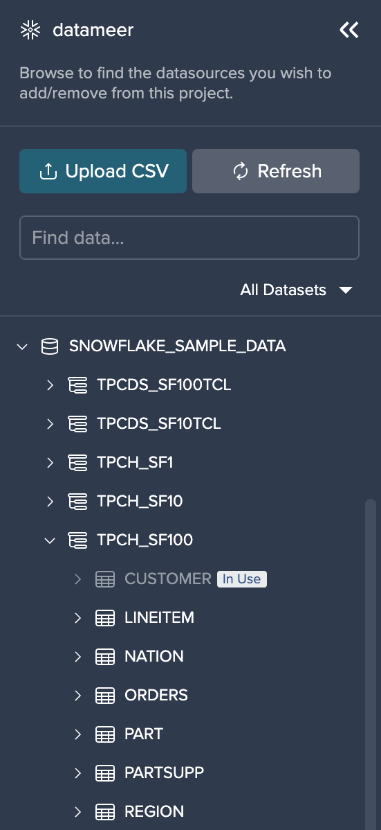
Data Browser#
Data Browser Overview#
The Data Browser provides all your Snowflake Schemas and datasets.
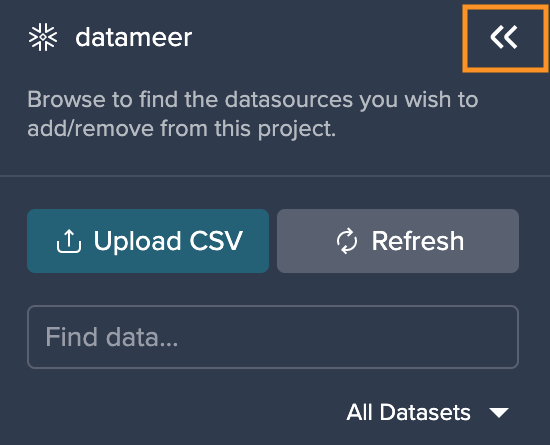
You can fade in or fade out the Data Browser by clicking "<<".
The Data Browser provides the following information:
- an 'Upload File' button to upload data from your device
- all of your Snowflake Warehouses, ordered alphabetically
- all of your Snowflake Schemas and datasets
- a filter option to browse more specifically through your data
The order within the Data Browser is the following:
- Snowflake Warehouses are sorted alphabetically
- Snowflake Schemas are sorted alphabetically
- tables are sorted alphabetically
- columns are sorted in the order defined in Snowflake's Schema
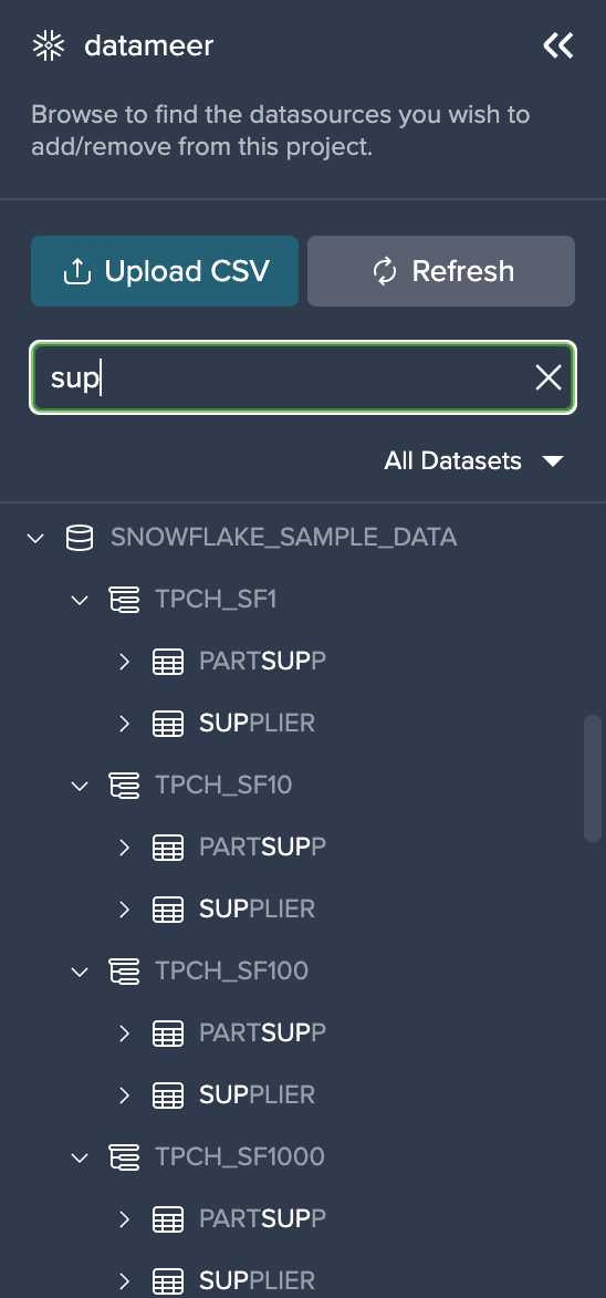
Browsing Datasets#
In order to find your needed dataset, you can enter your text in the search bar. Filtering is possible for databases, schemas and tables. Column filtering is not possible.
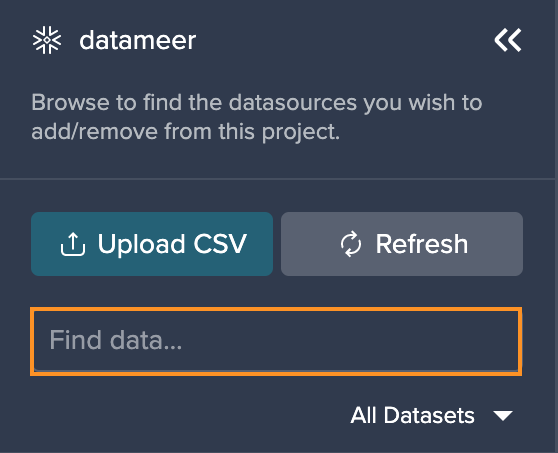
Find your matching entries listed below the search bar.
More Filtering Options#
You can filter the entries by the following criteria:
- "All Datasets": all available datasets are displayed
- "Added Datasets": shows added and in-use datasets for the actual Project
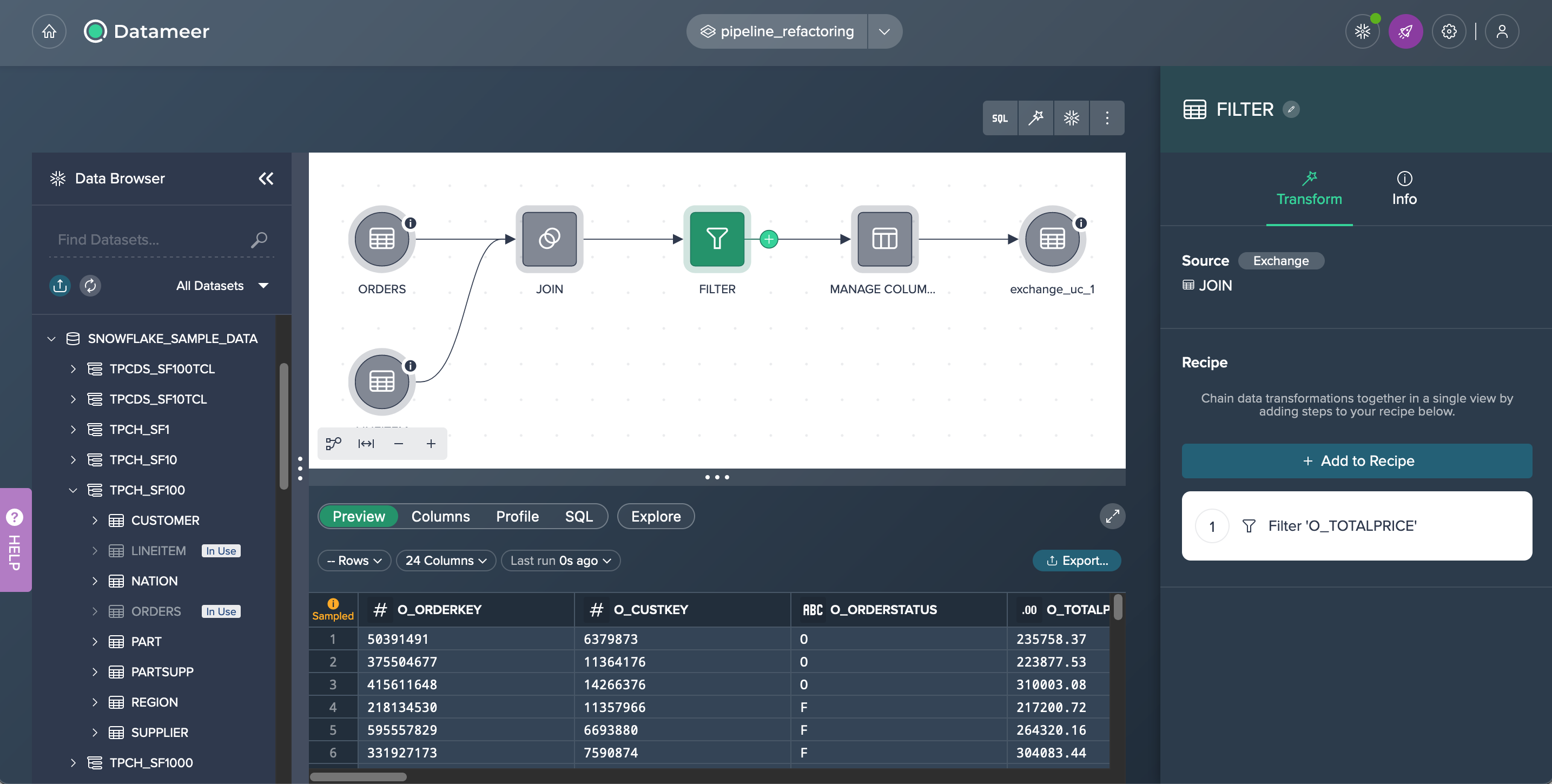
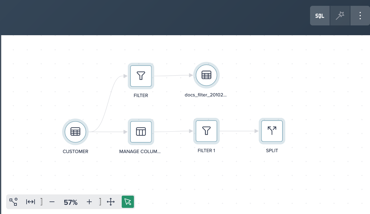
Flow Area#
The Flow Area visually represents your whole transformation pipeline, including data sources, transformations as well as deployed data sets.
The toolbar above the Flow Area is largely responsible for operating the Flow Area and allows you to open the SQL Editor, build new transformations and refresh used Snowflake sources.
Data Source Node Options#
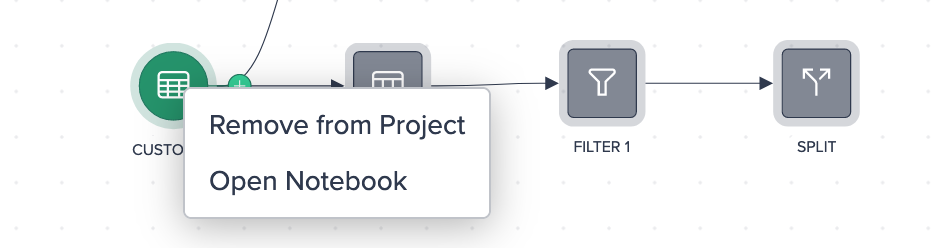
Starting from a data source node you can:
- remove the node from the Project (Note: But not simultaneously from your Snowflake instance)
- open the node in the Notebook
Transformation Node Options#
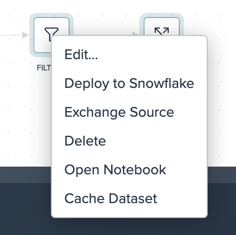
For a transformation node you can:
- edit the node
- deploy or re-deploy the node to Snowflake
- exchange the transformation source
- delete the node from the Project
- open the node in the Notebook
- cache the dataset
Deployed Nodes Options#
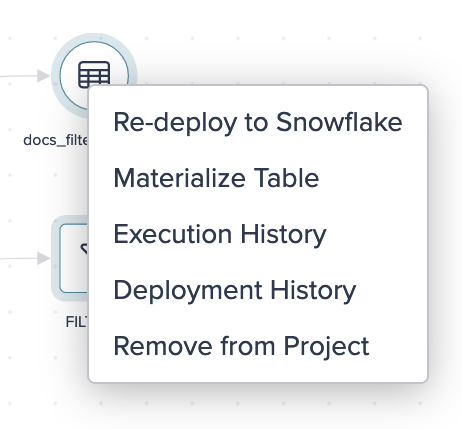
For a deployed node you can:
- deploy or re-deploy the node to Snowflake
- materialize a table
- show the Execution History
- show the Deployment History
- remove the node from the Project (Note: But not simultaneously from your Snowflake instance)
Scheduled Email Node Options#
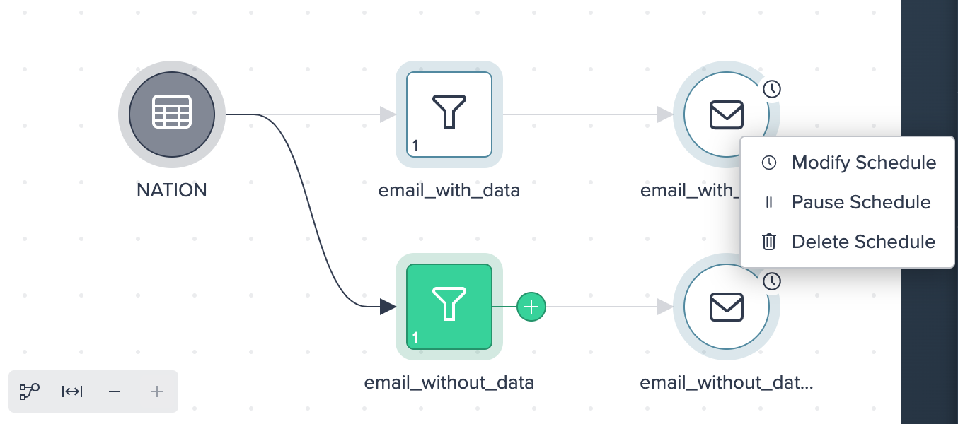
For a scheduled email node you can:
- modify the scheduling
- pause and resume the scheduling
- delete the scheduling
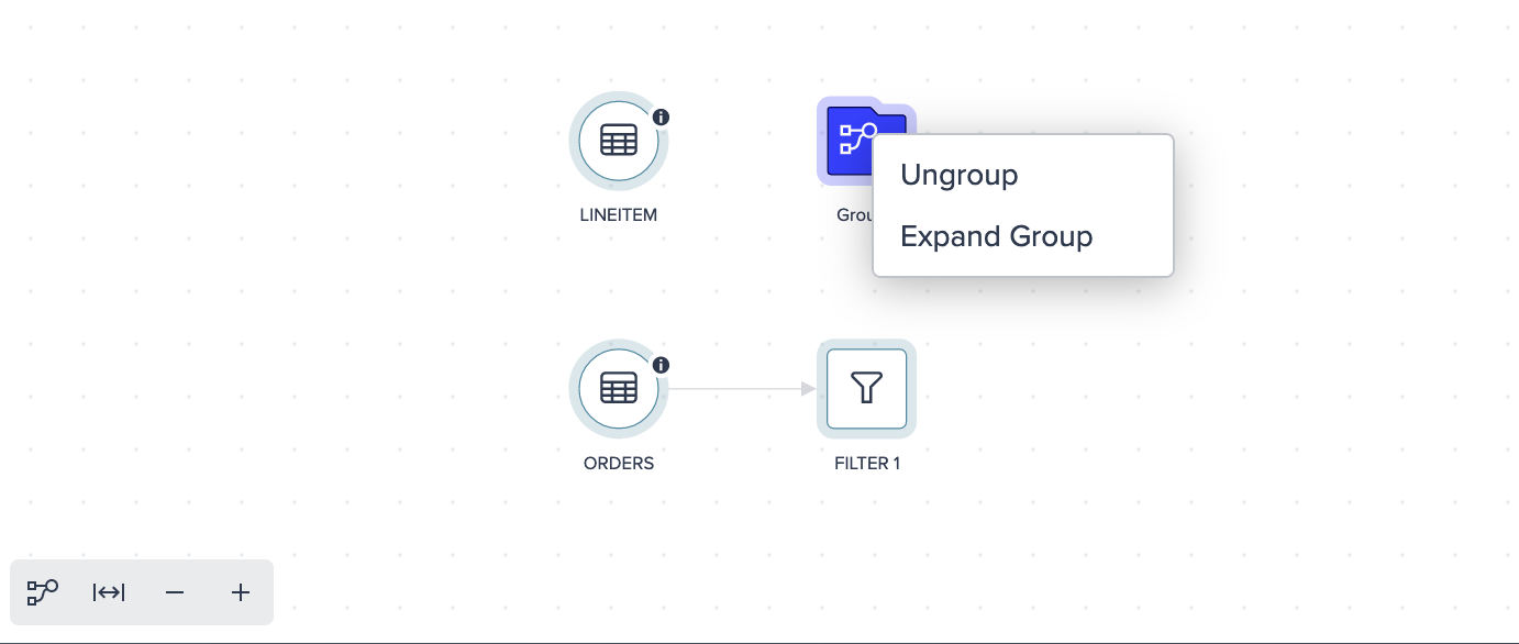
Grouping Node Options#
Once more than one node is grouped, you can do the following from the context menu:
- ungroup the grouped nodes
- expand the group and view all grouped nodes
Flow Area Visibility#
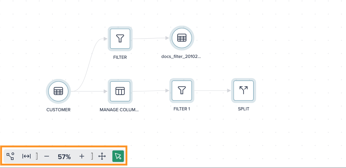
You can customize the display of your flow area by clicking on the different icons:
- hide unconnected nodes, only used nodes in the pipeline are displayed
- make the nodes fit to the size of the Flow Area
- zoom in and zoom out
Data Grid#
Data Grid Overview#
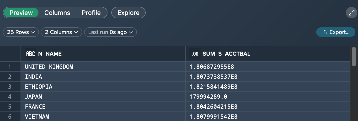
The Data Preview area enables you to view a data preview, explore the columns within a dataset and metadata as well as several exploration features. You can also share your data via email, to a Google Sheet or download a CSV.
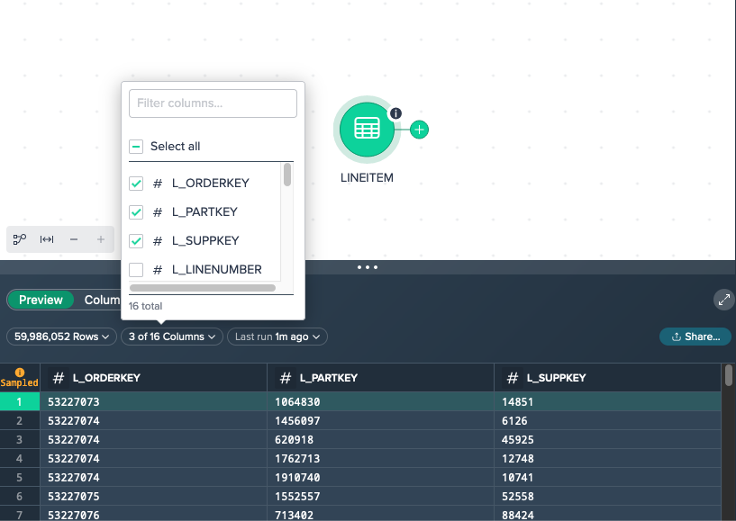
To view a data preview of the actual data and get information about the rows and columns, click on "Preview".
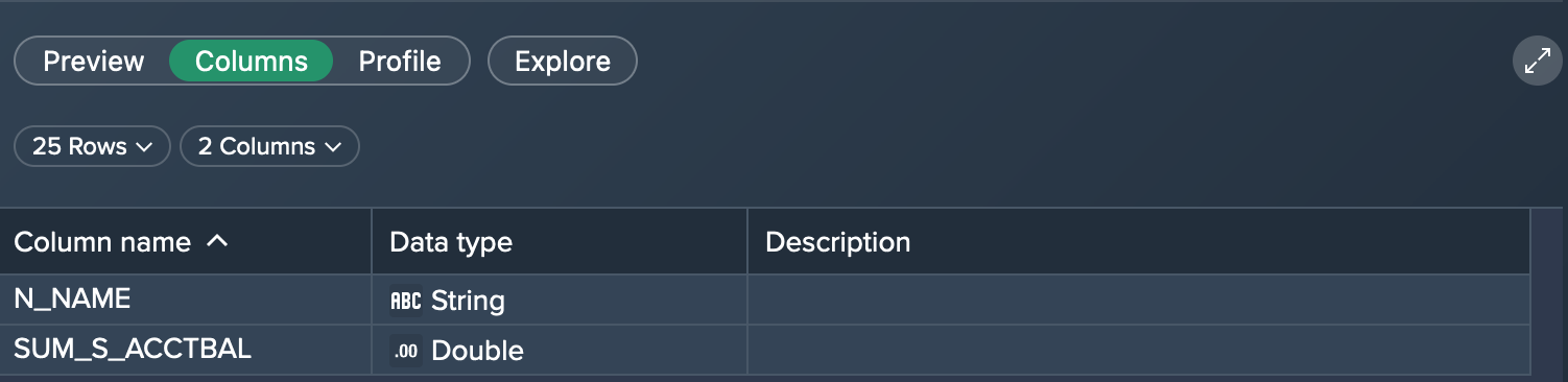
To explore the columns of a dataset, click on "Columns". This view presents the column names (table schema), their data type as well as metadata (optional).
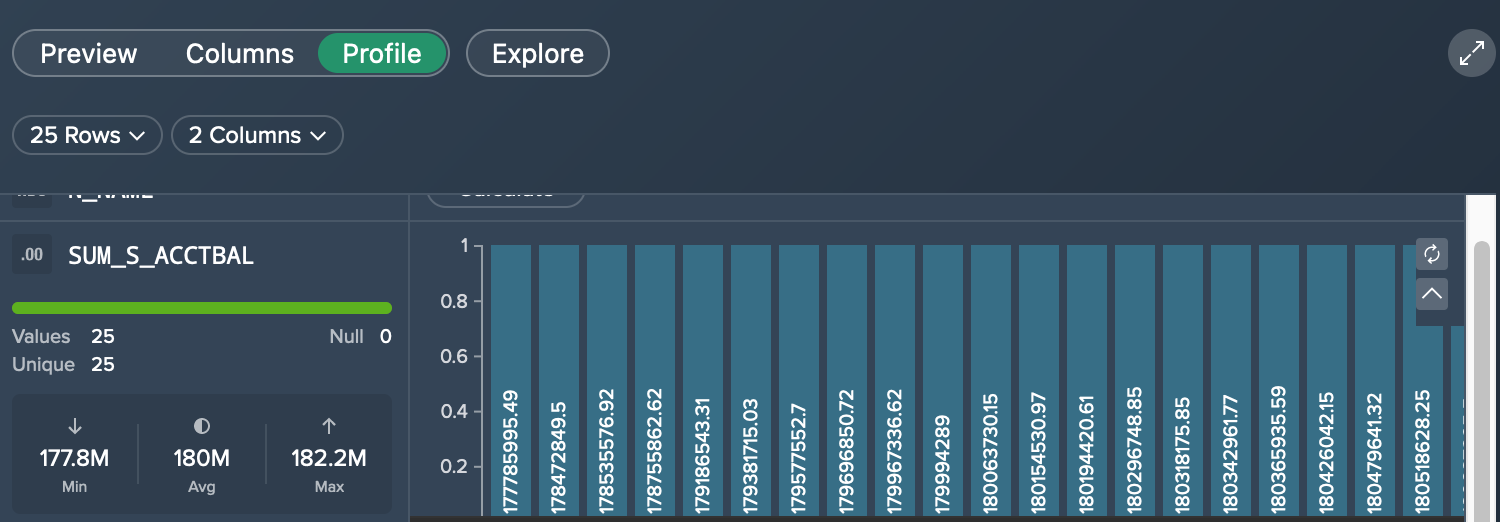
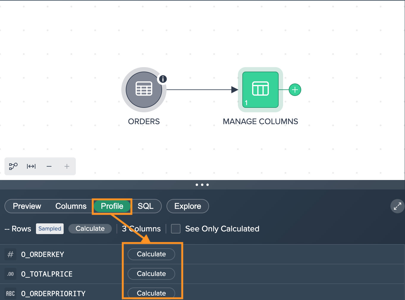
To view the profile information such as column metrics, click on "Profile".
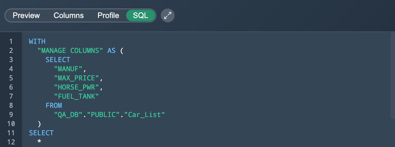
To view and copy the SQL query for views, click on "SQL".
To keep the most important things in view, you can limit the number of columns by selecting the columns. For that, click on the 'Columns' drop-down and select the needed columns. Columns that have been hidden once can be shown again later here.
Column Metrics#
You can investigate column metrics in the 'Profile' tab for any data type. For each column a statistic can be shown.
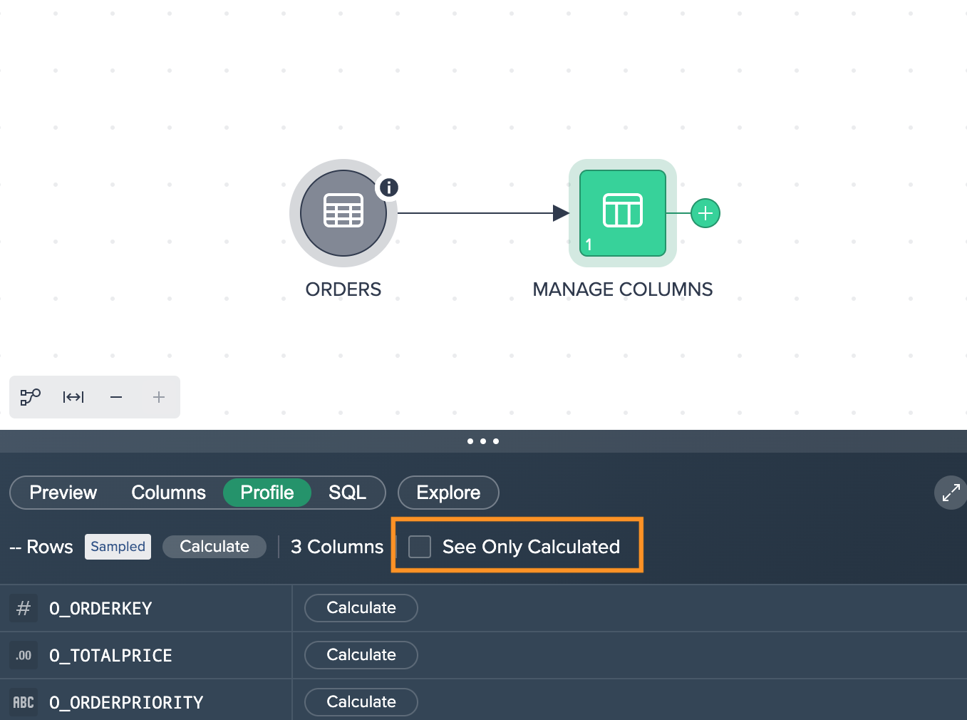
To perform calculations, switch to the tab "Profile" in the Data Grid. Click on "Calculate" in the required columns. The metric is displayed for the respective column.
To calculate all columns at once, click on "Calculate".
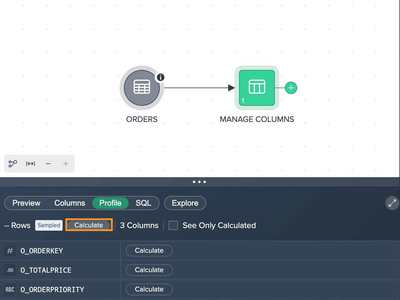
You can also display only the calculated columns. For that, hit the checkbox "See Only Calculated". All calculated metrics are shown.
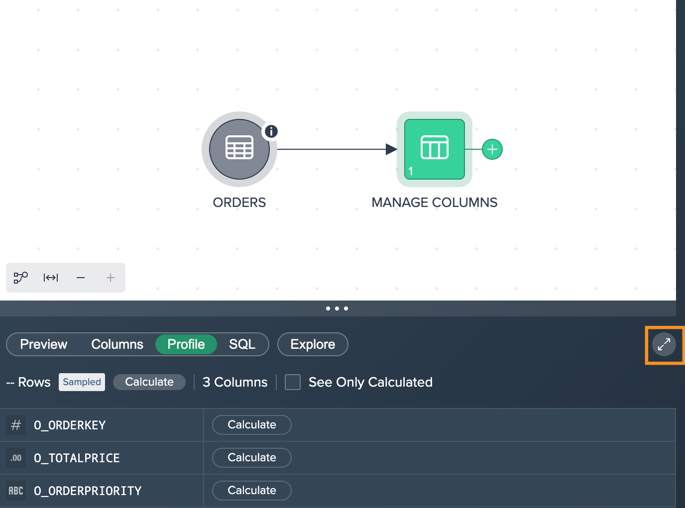
To enlarge the metrics view, click on the 'Maximize' button. You can go back to the minimized display, when clicking the button again.
As a calculation result, each metric shows:
- Data type and column name
- a green loading bar, that visualizes the ratio between available values and missing entries in the column, e.g. you have 500 values but 500 entries are missing, the bar would be half green and half red
- total number of values and total number of empty entries
- total number of unique values, if 5,000 values are calculated in the preview, a max. of 5,000 values can be reached. If there are only 5 different values out of 5,000 possible values, the 'Unique' would show '5'
- values for minimum, average and maximum
- a visualization, depending on the data type
Clicking the 'Minimize' button provides information for unique and null value amount as well as the minimum, average and maximum value.
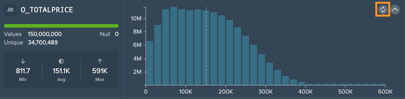
To refresh the calculation, click on the 'Refresh' button next to the graphics.
Examples
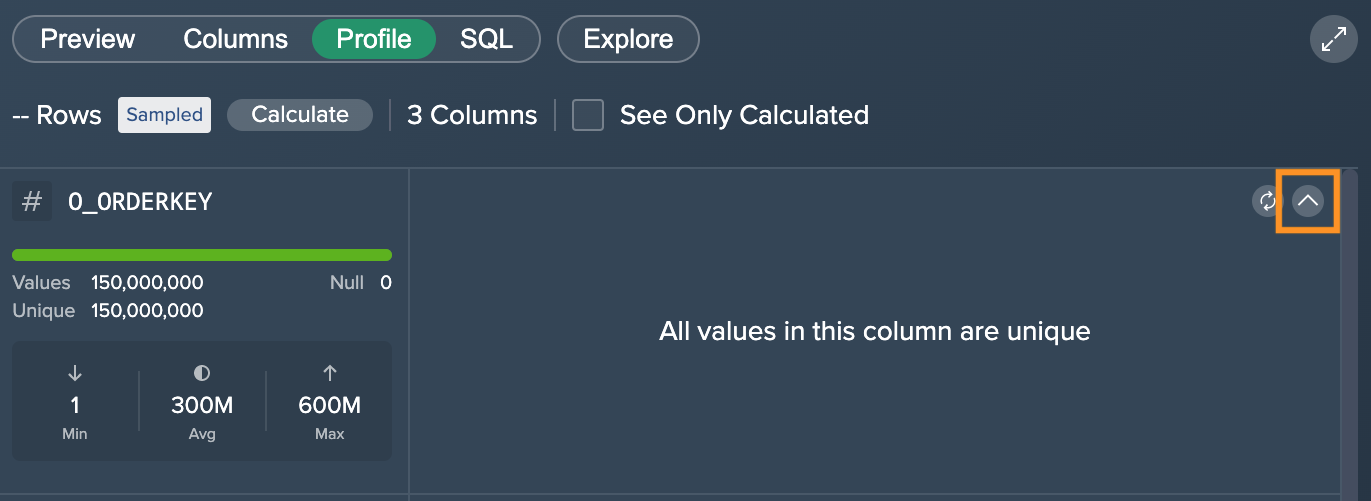
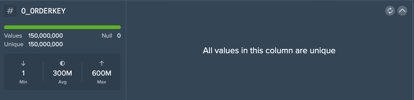
Datatype: INTEGER
Since this dataset is sampled, the column "0_ORDERKEY" contains 150,000,000 values in total, 0 empty/ null values and 150,000,000 unique values. The minimal value is 1, average is 300,000 and maximum is 600,000,000. Since we have unique values only, no graphic is being presented in this case.
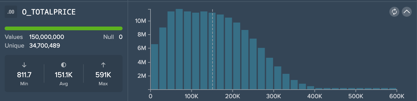
Datatype: DECIMAL
Since this dataset is sampled, the column "0_ORDERPRICE" contains 150,000,000 values in total, 0 empty/ null values and 34,700,489 unique values. The minimal value is 811.7, the average is 151K (rounded) and maximum is 591K (rounded). The graphic shows the amount of values that belong to a specific price. The dashed line meanwhile marks the average.
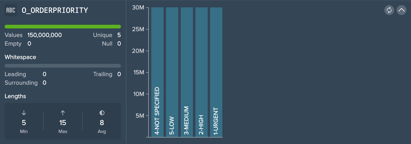
Datatype: STRING
Since the dataset is sampled, the column "0_ORDERPRIORITY" contains 150,000,000 values in total, 5 unique values and 0 empty/ null values. Whitespace is 0 and indication for the STRING length is minimum 5, 15 for maximum and an average of 8. The graphic shows the 5 unique STRING values and the amount of usage in this dataset.
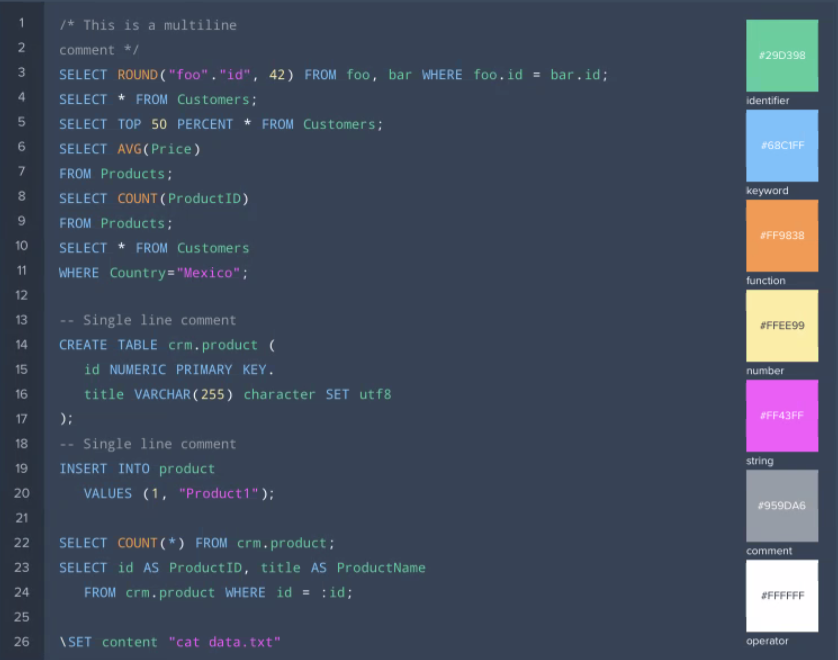
SQL Syntax#
The SQL syntax is highlighted to identify the single syntax expressions. Find the following highlighting in the SQL Editor:
Inspector#
The Inspector contains all information about the actual dataset/ table/ warehouse/ Project that is selected.
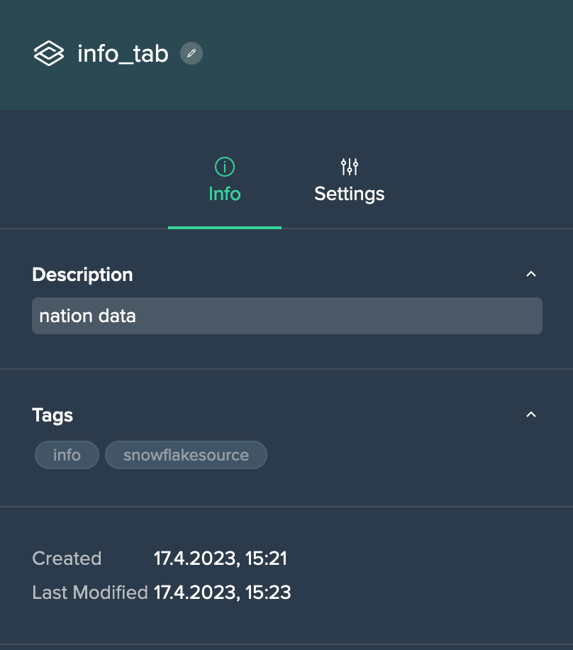
Project 'Info' Tab#
The Project's 'Info' tab provides the following information:
- Project description: view and add a description
- Project tags: view and add tags
- date and time when the Project has been created
- date and time then the Project has been modified
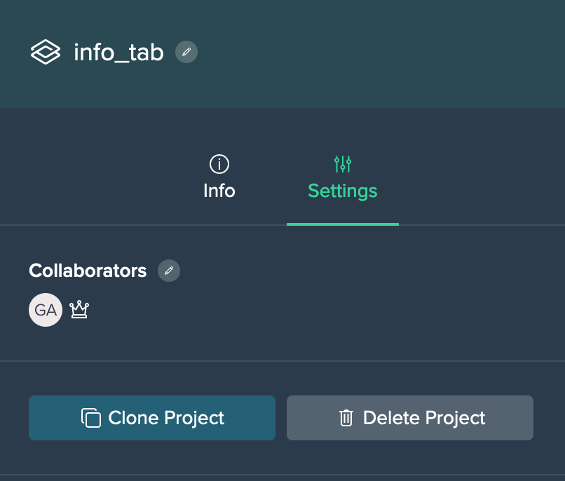
Project 'Settings' Tab#
The Project's 'Settings' tab provides the following information:
- collaborators
- option to clone the Project
- option to delete the Project
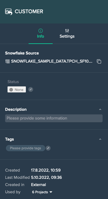
Source Node 'Info' Tab#
The source data 'Info' tab provides the following information:
- Snowflake source as fully qualified name
- status: view and add a status
- description: view and add a description
- tags: view and add tags
- date and time when the source asset has been created
- date and time when the source asset has been modified
- 'created in' information
- used by the amount of Projects and the associated Project list
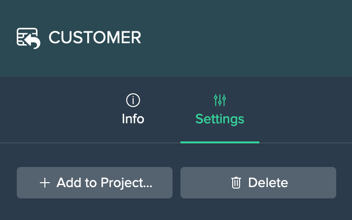
Source Node 'Settings' Tab#
Each source node 'Settings' tab provides the following options:
- add the node to a Project
- delete the node (from Snowflake and Datameer)
Transformation Node 'Info' Tab#
Each transformation node 'Info' tab provides the following information:
- description: view and add a description
- transformation node owner
- tags: view and add tags
- date and time when the transformation node has been created
- date and time when the transformation node has been modified
![]()
Datameer's AI features enable you to generate a description simply by clicking on the "Auto-generate Description" icon next to the 'Description' section.
Transformation Node 'Transform' Tab#
Each transformation node 'Transform' tab provides the following information:
- the associated source node
- a button to exchange the source node
- the receipt list with all transformations
- a button to add a transformation to the receipt
![]()
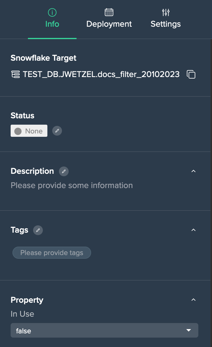
Deployed Node 'Info' Tab#
Each deployed node 'Info' tab provides:
- Snowflake target with link
- status information and status editing option
- description and description edit option
- tags and tag edit option
- set property option
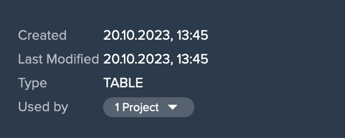
- meta data: creation date and time, last modified date and time, table/view, amount of usage in Projects
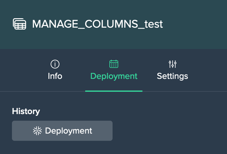
Deployed Node 'Deployment' Tab for Views#
Each deployed view node 'Deployment' tab provides:
- a Deployment History button
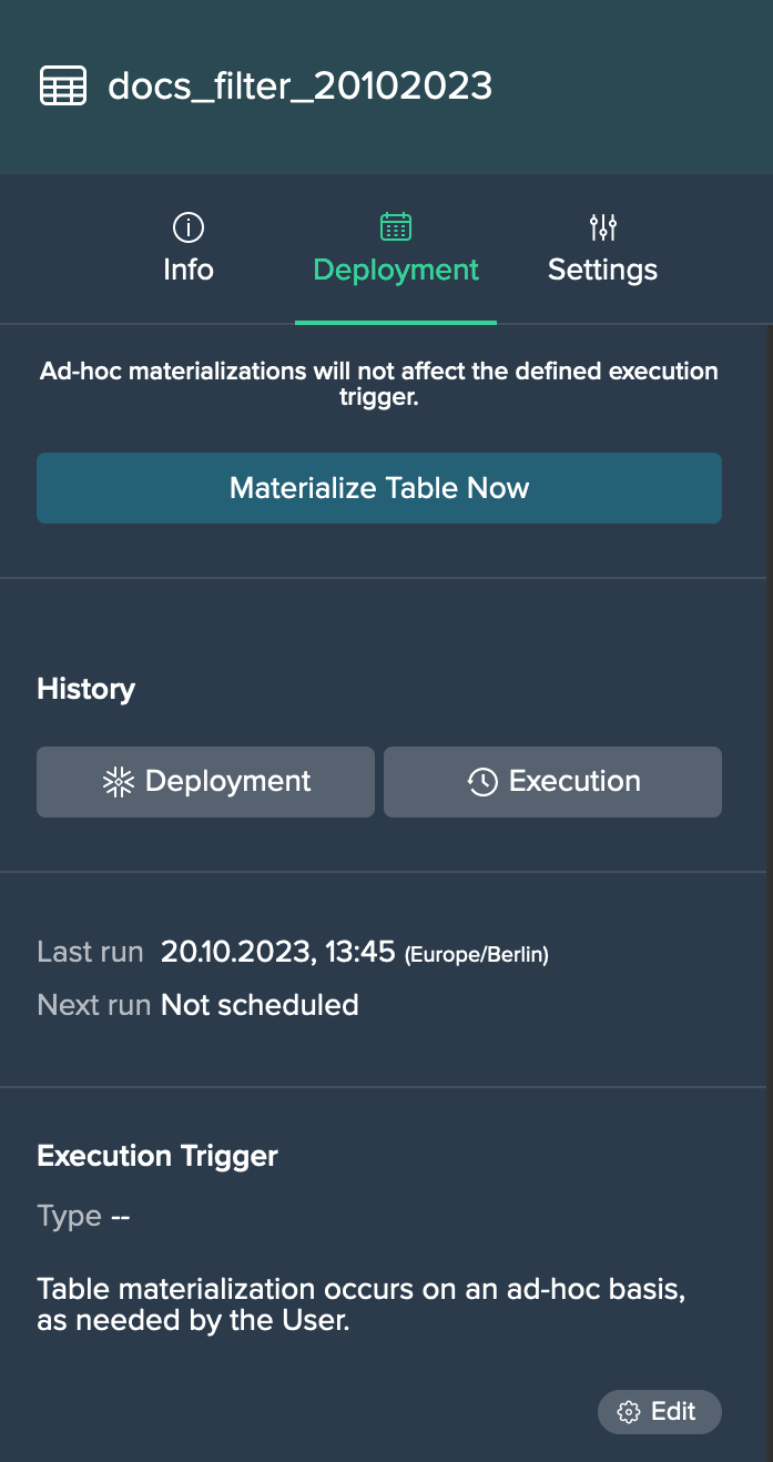
Deployed Node 'Deployment' Tab for Tables#
Each deployed table node 'Deployment' tab provides:
- table materialization option
- Deployment History button
- Execution History button
- date and time information for the last run (with status) and the next run
- execution trigger configuration
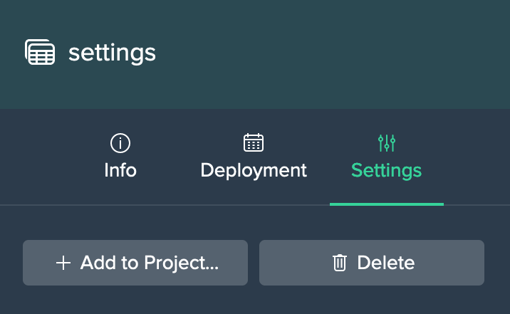
Deployed Node 'Settings' Tab#
Each deployed node 'Settings' tab provides the following options:
- add the node to a Project
- delete the node (from Snowflake and Datameer)