Exploration Use Cases
These use cases might help you to understand the usage of the exploration feature. Both use cases focus on large data sets that are automatically sampled when working on them in Datameer. For that remember that data sets that are smaller than 100,000 records are not sampled.
Validating Data Sets#
This use case demonstrates how to perform a statistical survey to determine the sales rate of high-priced products. The objective is achieved by utilizing the following functionalities within Datameer:
- transformation operation FILTER
- data validation via exploration
Scenario#
A clothing company sells a lot of goods via an online store and would like to have an overview list ready of all sold products that have a price higher than 500,000 §. For that they have a table containing 150 billion records in their Snowflake. You - as the analyst - was given the part to create a temporary list of the required products to solve the question.
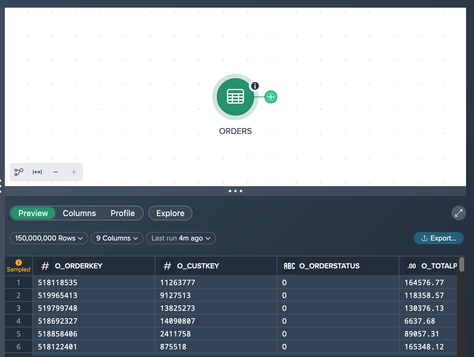
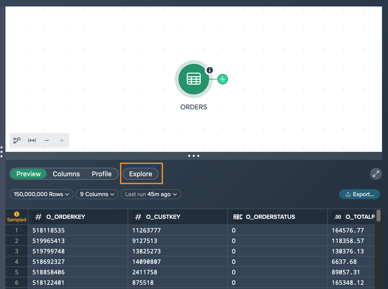
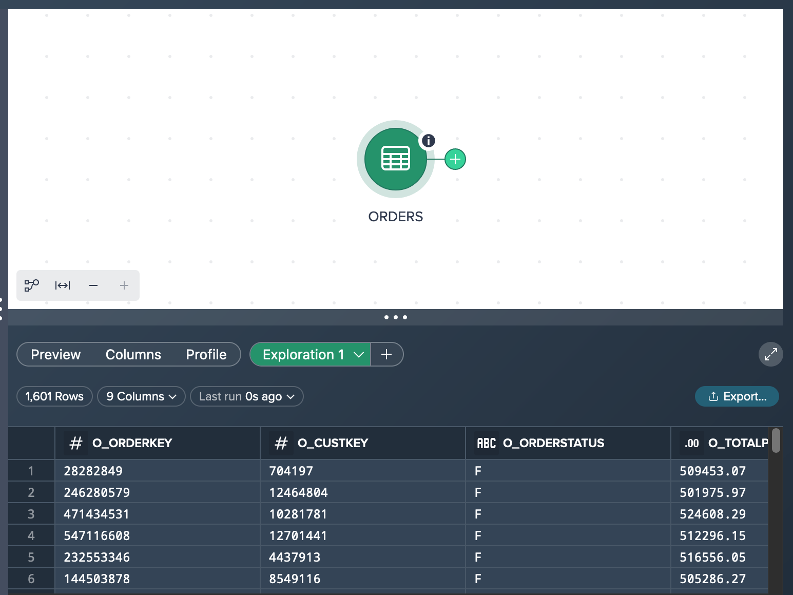
Let's assume you have added the source data set 'ORDERS' (including 150,000,000 records) to the Workbench in a new Project. What you see in the Flow Area is the source node 'ORDERS' that is marked as a sampled data set. The preview in the Data Grid below presents 100 rows of the sample data.
Trying to figure out how many products +500,000 $ are contained you have two options:
- filtering the 'ORDERS' dataset (based on sample data)
- running an exploration on the 'ORDERS' data set (based on full data)
Via Filtering Transformation on Sample Data#
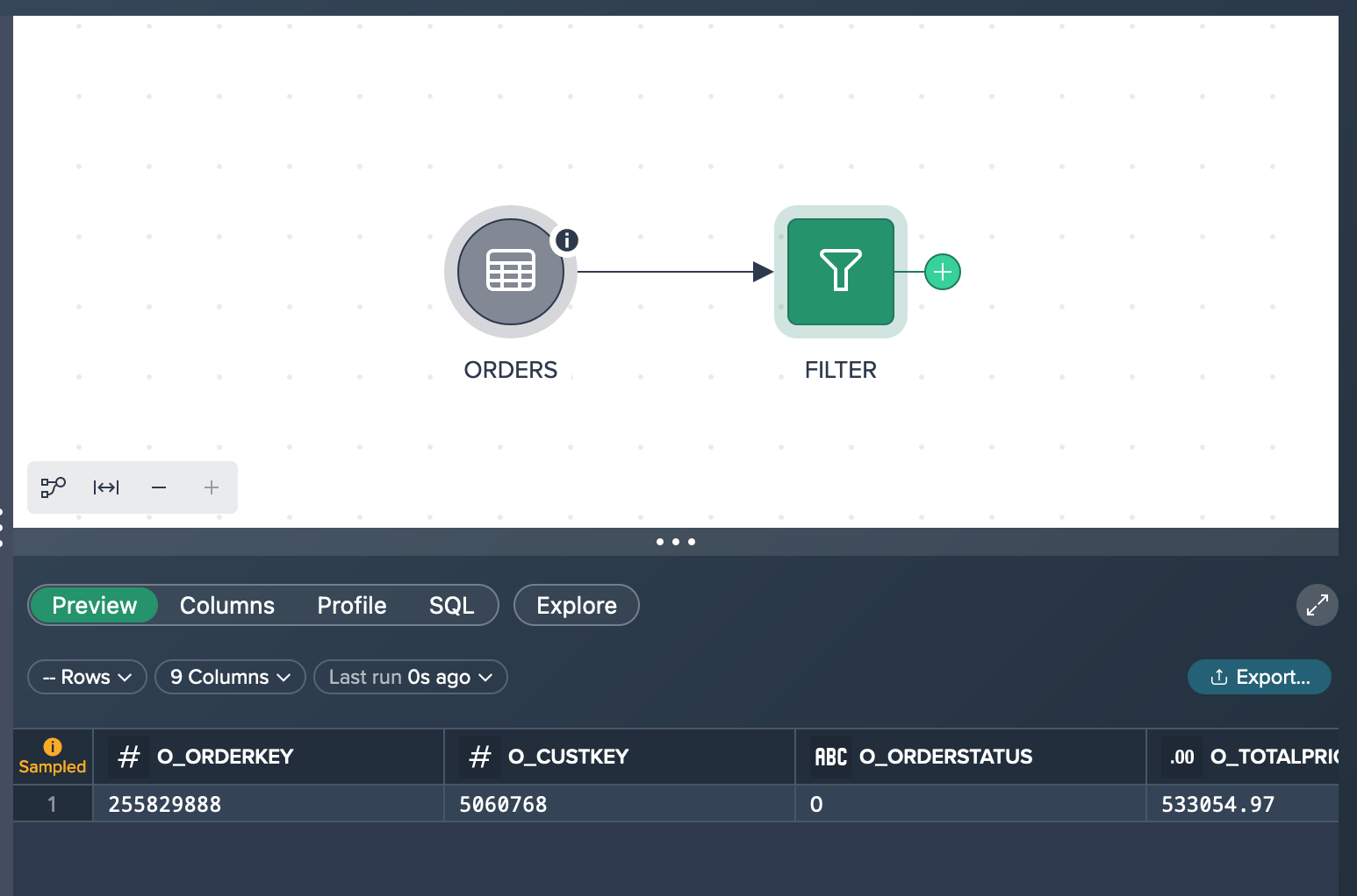
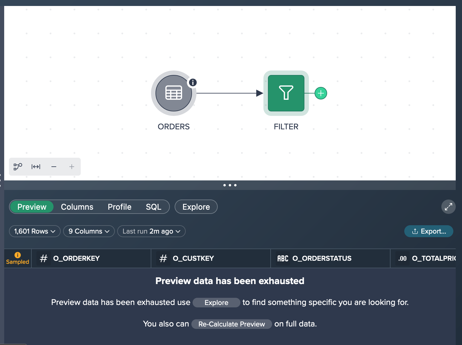
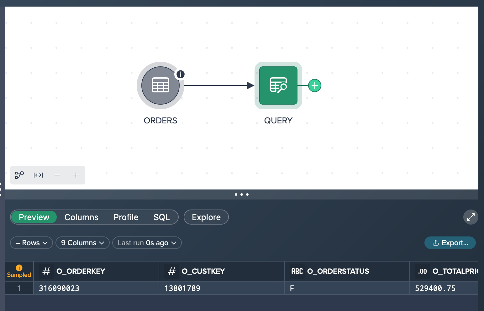
Filtering the data set results in a transformation 'FILTER' node with a data preview that bases on on the sampled source data set. In your specific scenario, you observe that the result shows only one row, indicating that there is only one product with a price higher than 500,000 $. However, this outcome is not aligned with your expectations, causing concern and raising doubts about its accuracy.
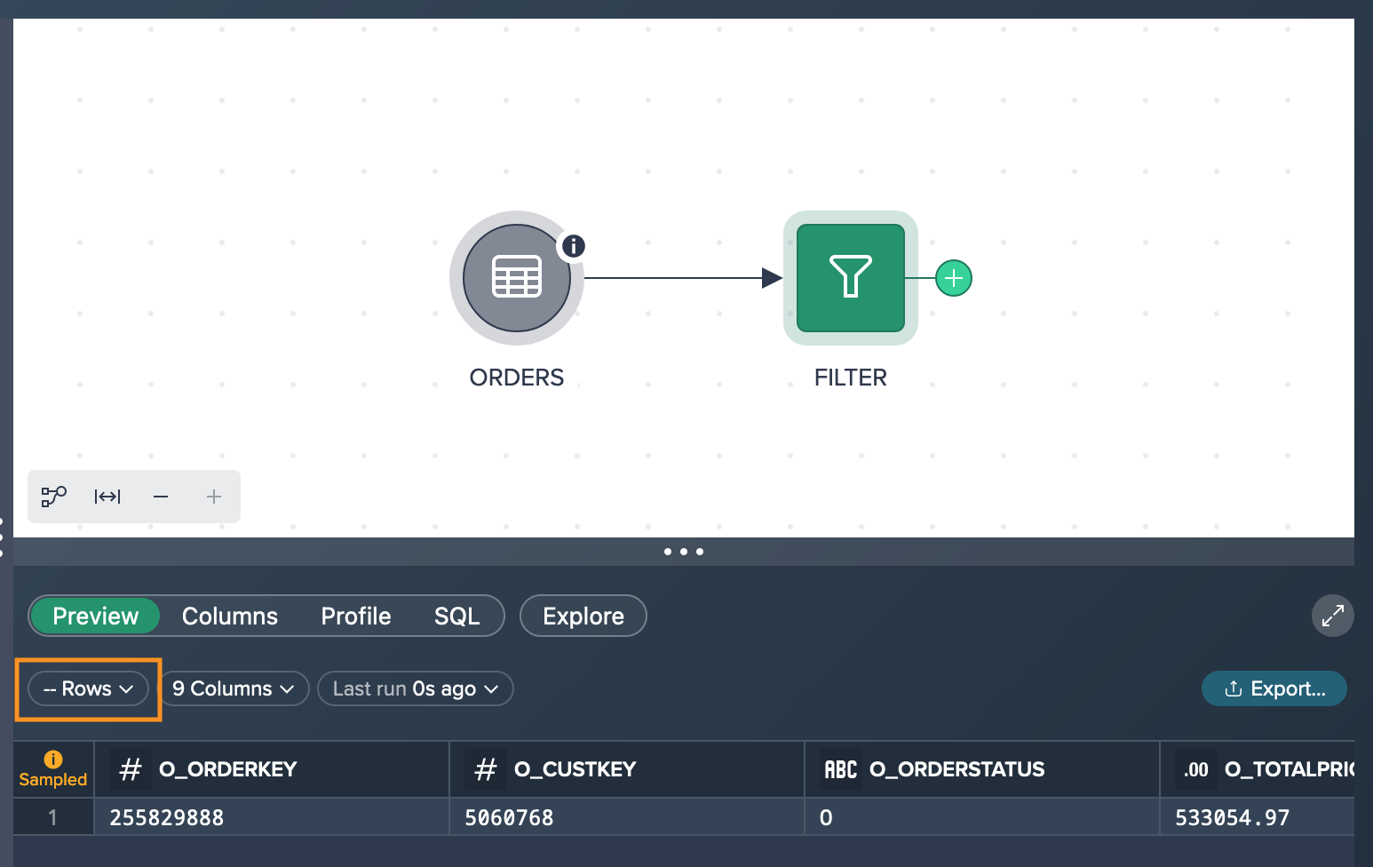
When you click on the 'Rows' option, a query is executed to determine the exact number of records that meet your specified criteria. This query counts the actual amount of records in the dataset that correspond to the conditions you have set. This provides a more accurate and reliable count of the records that meet your criteria, giving you a clearer understanding of the data that matches your requirements.
If you want to view more preview rows and see different records than those displayed in the sampled preview, you can refresh the data. By refreshing the preview, the data is updated, allowing you to see a new set of records. This enables you to explore and analyze a wider range of data, providing a more comprehensive understanding of the dataset beyond the initially sampled records.
Be aware that it might be possible to see no matching records because the sample data might not include all relevant records in the preview. At this point you can start an exploration or re-calculate the preview on full data. Both can take a significant time, depending on the data set size.
In our case you decide to take the time to run against full data and finally get the full data set filtered. Since you have only 1,601 matching records, no sampling is necessary and the preview presents 100 of the 1,601 rows.
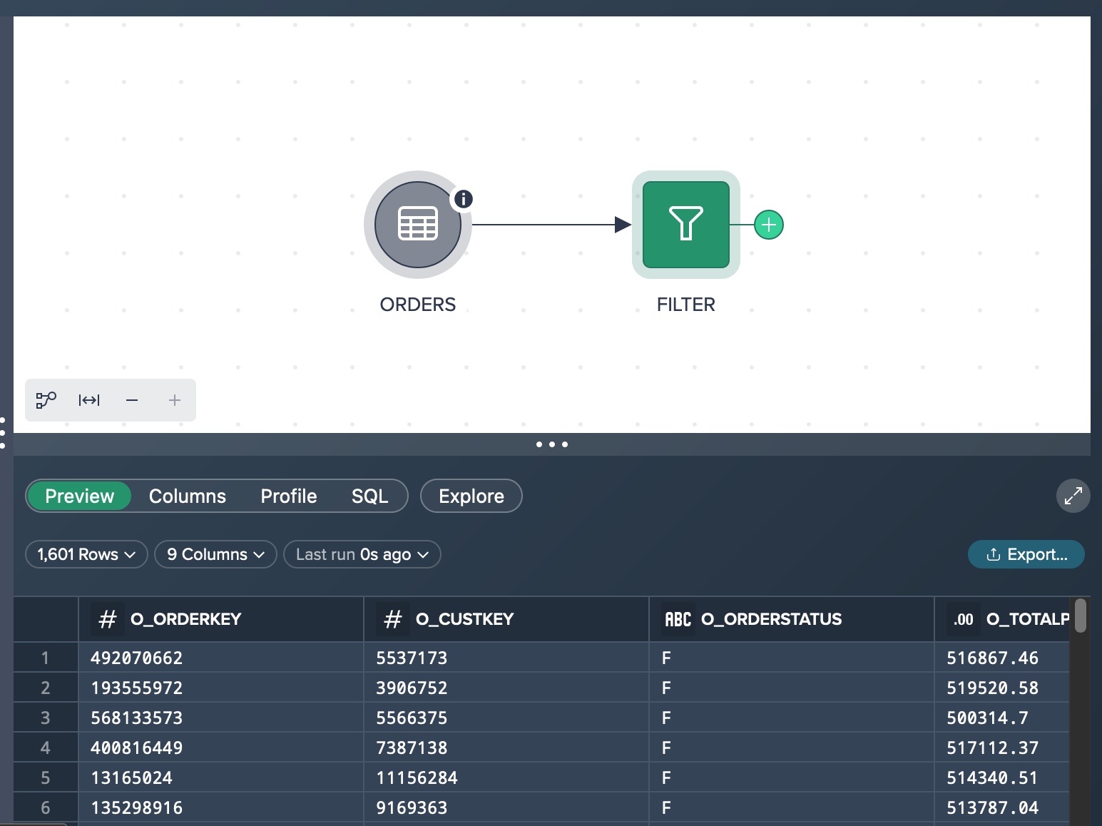
Finally you have a 'FILTER' transformation node that contains 1,601 records of products that have a price higher than 500,000 §.
Via Quick Exploration Validation on Full Data#
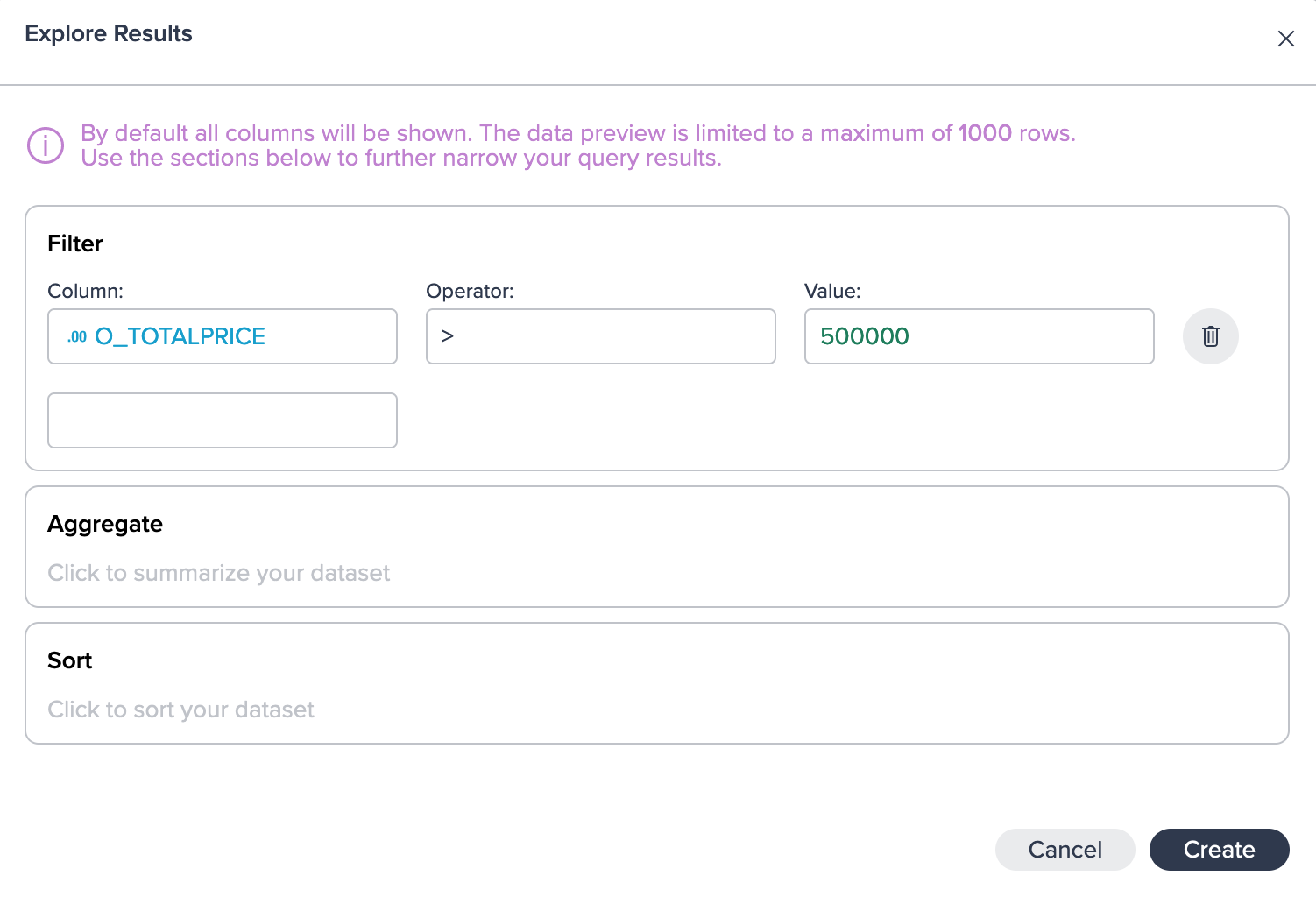
A quick and easy way to reach your goal is to explore the data set via the 'Explore' feature on top of the Data Preview. You click on 'Explore' and the 'Explore Results' dialogs opens.
After applying the desired filter and executing the query, you observe that the total number of rows matching our criteria is 1,601. In the Data Preview, you are presented with a subset of the results, specifically 1,000 records. It's important to note that this exploration is performed using the complete dataset, ensuring accurate and comprehensive results. By achieving these outcomes, you have successfully accomplished your intended goal.
Converting the Exploration to a Transformation#
If desired, you have the flexibility to convert your intermediate exploration into a transformation and integrate it into your pipeline within the Flow Area. This can be achieved by either dragging and dropping the exploration tab directly into the Flow Area or by using the context menu and selecting the 'Convert to Transformation' option.
Ad-Hoc Data Analysis#
This use case demonstrates how to create an ad-hoc analysis for forecast calculation of shipping modes. The objective is achieved by utilizing the following functionalities within Datameer:
- aggregating a joined data set
- ad-hoc exploration
Scenario#
A clothing company sells a lot of goods via an online store and wants to find out how many orders have been shipped by truck in order to forecast a truck load occupancy rate. For that they have a table containing more than 600 billion records in their Snowflake. You - as the analyst - was given the task to solve the question whether the estimated amount of shipped products by truck fits the expectations.
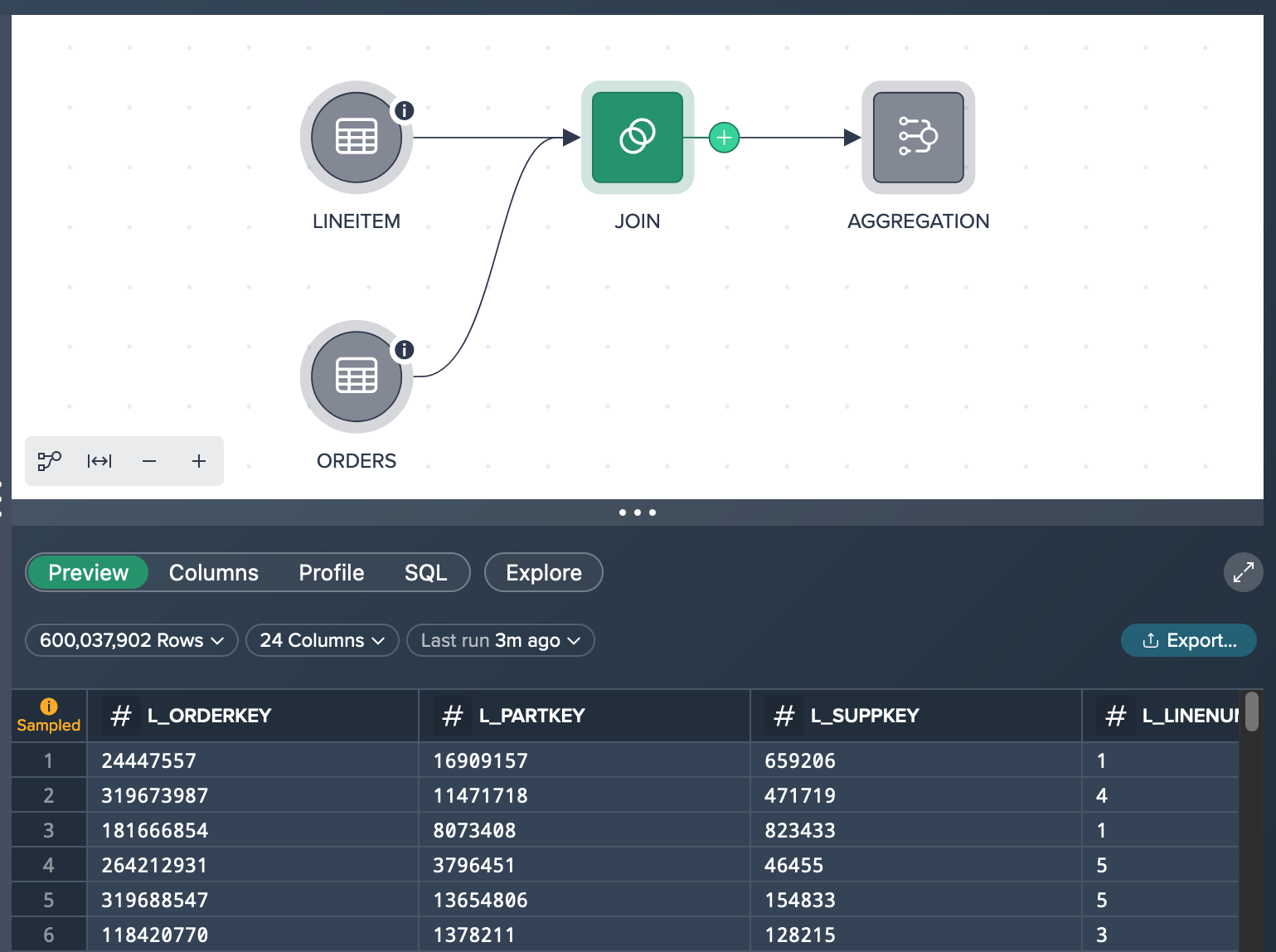
Let's assume you already added the data set 'ORDERS' that has 150,000,000 rows with records and 9 columns in total as well as the data set 'LINEITEM' that has 600,037,902 records and 16 columns. You performed the light data prep operation 'JOIN' to join the orderkeys. After calculating the row count, the JOIN node contains 600,037,902 records.
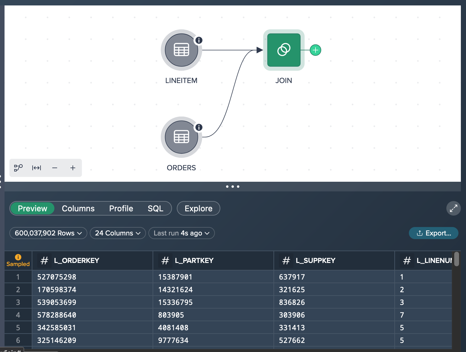
What you see in the Workbench is both source nodes (already sampled down to 100,000 records because of their large individual size). and the JOIN node. The JOIN node preview in the Data Grid below the Flow Area presents 100 rows of the sampled JOIN data set.
Trying to reach your goal you have two options:
- aggerating the 'JOIN' dataset (based on sample data)
- running an exploration on the 'JOIN' data set (based on full data)
Measuring the 'TRUCK' Count via Aggregation Operation on Sample Data#
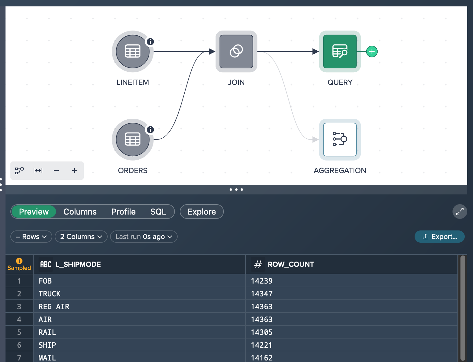
You run the aggregation operation via the operation stack and group by the shipmode column and measure the count.
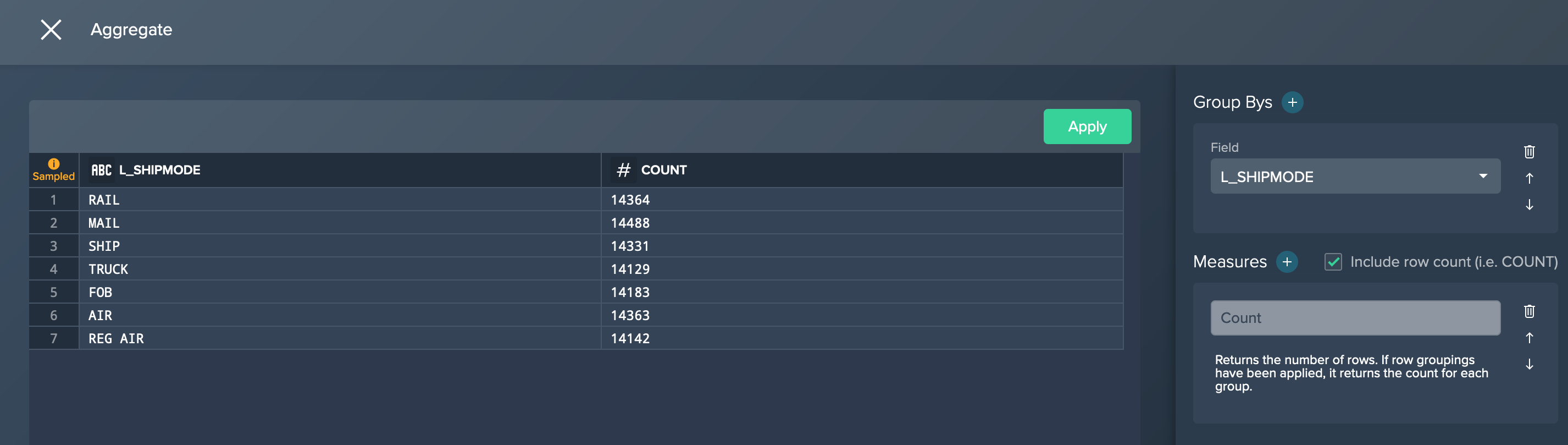
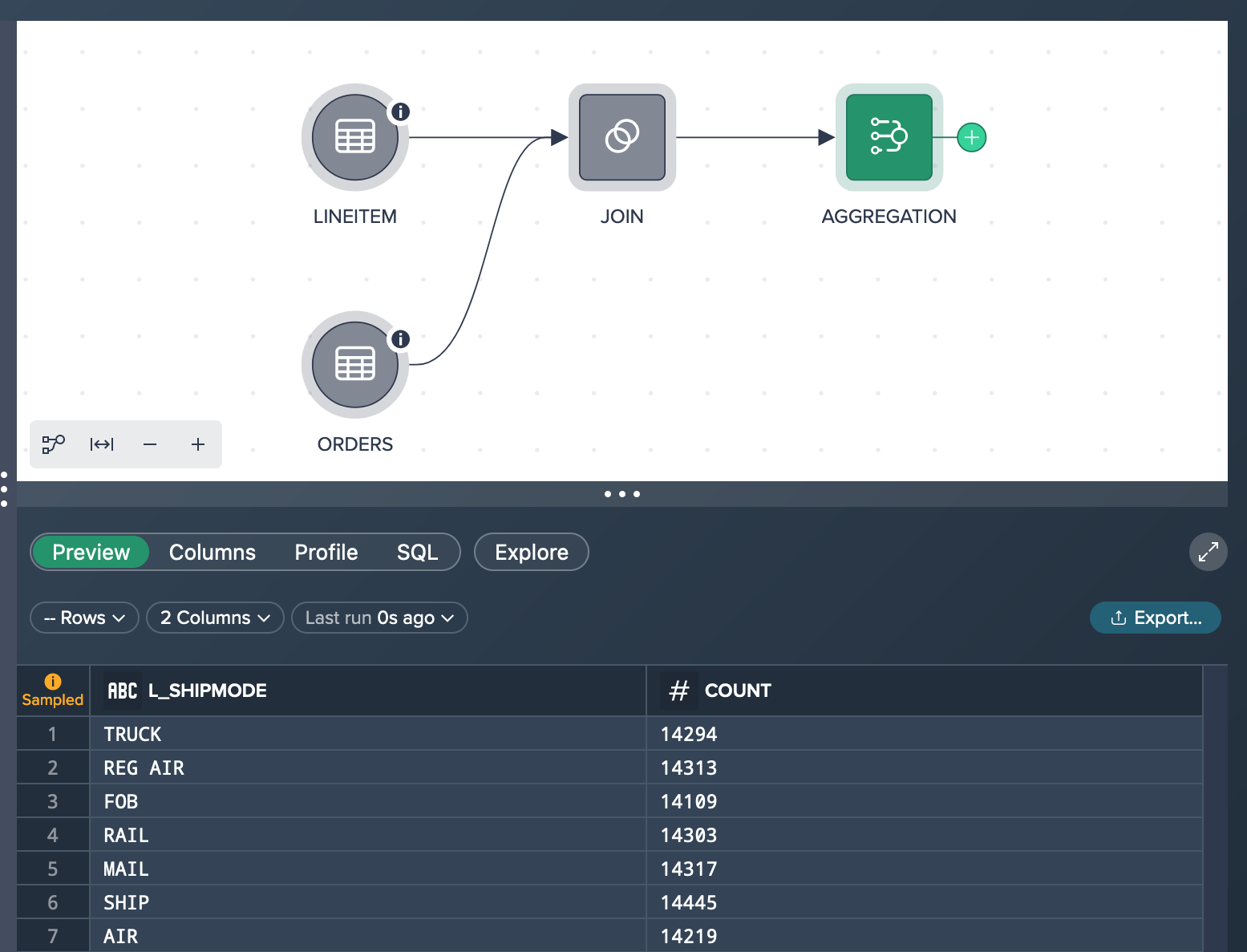
As a result the preview shows e.g. for the shipmode 'TRUCK' 14,294 orders. Usually, the Data Grid preview would present 100 rows of the aggregation node but in your case you only have 7 lines because there are only 7 shipping modes in the data set.
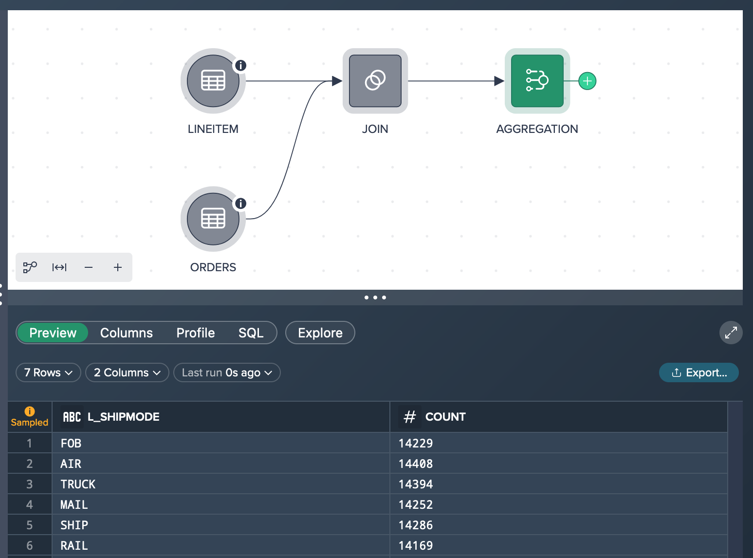
Upon rerunning the preview, you observe inconsistent results such as 14,394 orders by truck in one run and 14,354 in another, and so on. This discrepancy appears significantly lower than expected. To address this issue and perform an ad-hoc analysis based on the complete dataset, you can leverage the exploration feature discussed in the upcoming chapter. The exploration feature allows you to explore the data comprehensively and gain more accurate insights for our analysis.
Measuring the 'TRUCK' Count Via Exploration Query on Full Data#
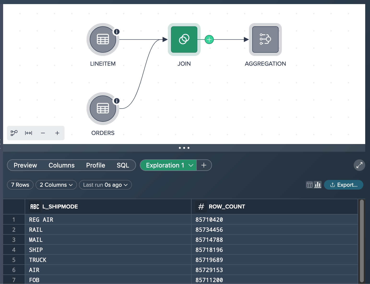
Starting from the 'JOIN' node you click the 'Explore' pill to configure the 'Explore Results' dialog according to your needs: Group by the 'L_SHIPMODE' column and measure the row count.
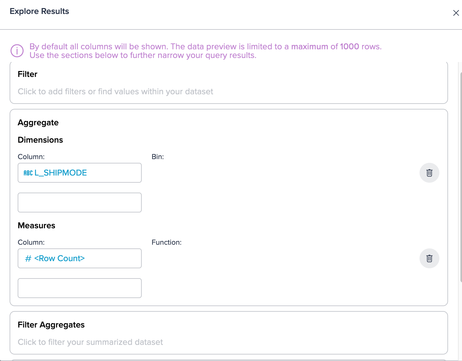
As a result, the 'Exploration 1' tab displays all seven shipmode rows along with the corresponding true row count value for each shipping mode. Specifically, when checking the 'TRUCK' row, you find a total value of 85,719,689. This information allows you to gain a comprehensive understanding of the dataset and provides accurate statistics for further analysis related to shipping modes, in your case especially for the shipping mode 'TRUCK'.
At this stage, you have the option to convert the exploration into a transformation, which enables you to expand your workflow pipeline. This transformation can be easily shared with a colleague who is currently working on the subsequent stages of the pipeline. By converting the exploration to a transformation, you can seamlessly pass on the refined and validated data processing steps to your colleague, facilitating smooth collaboration and continuity in the pipeline workflow.