Pivoting Data

Pivoting transposes rows to columns in order to group and aggregate data display. This is useful, for example, in datasets where you want to use just a subset of values from a column dimension, view different aggregations of the same column and the same aggregation of different columns, or simply to select more than one measure to easily group and compare values. ][Pivot tables can be generated from samples and by querying against a complete dataset. The pivot inspector is interactive, so once a pivot sheet is created you can test and update your results iteratively.

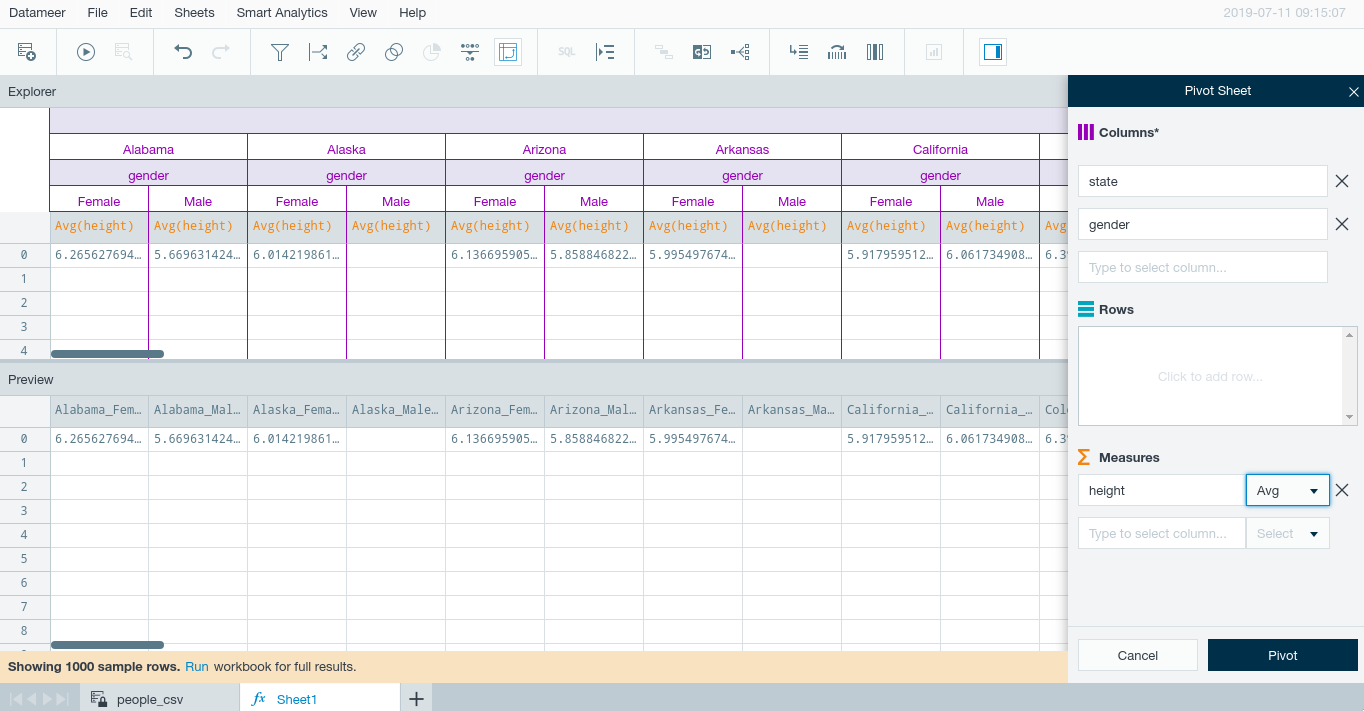
For example, in a Workbook that includes height, weight, age, gender, and state of residence for a set of individuals living in the United States, you could choose just certain states as the first column grouping, gender as the second column aggregation, then weight as the measure with average as the operator to yield the average weight by gender for the selected states.

Depending on the measure being used, supported aggregations are:

• ANY - returns any value in the group
• AVG - average of the values in a group for numeric values
• COUNT - number of elements in a group
• MAX - maximum of the values in a group for numeric values
• MIN - minimum of the values in a group for numeric values
• STDEV - statistical standard deviation inside the group for numeric values
• SUM - sum of the values in a group for numeric values
• VAR - statistical variance in the group for numeric values
• FIRST
• LAST

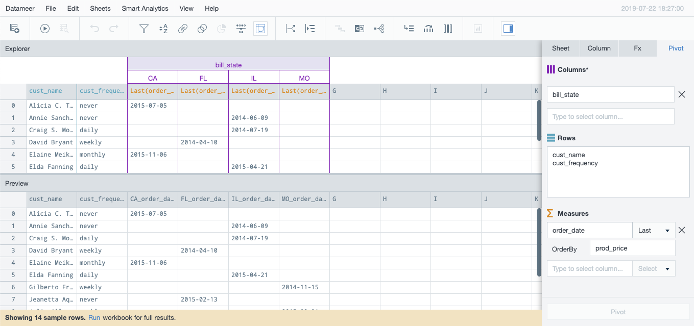
First and last are special functions that compute the first or last element inside a group given a specific order. For example, given the grouping by state and gender, you could select weight as measure with first as the operator and height as the OrderBy criteria to yield the weight of the tallest person per state by gender.

Creating a Pivot

To create a pivot:

1. In the active sheet, select Pivot from the Edit menu, or click the Pivot icon on the toolbar.
2. A new sheet will open in the pivot view with an Explorer at the top for visual display of the results, and a Preview table at the bottom.

3. In the Pivot Sheet dialog to the right, select one or more Columns on which to pivot and aggregate. Aggregation is hierarchical in the order of columns selected.

   

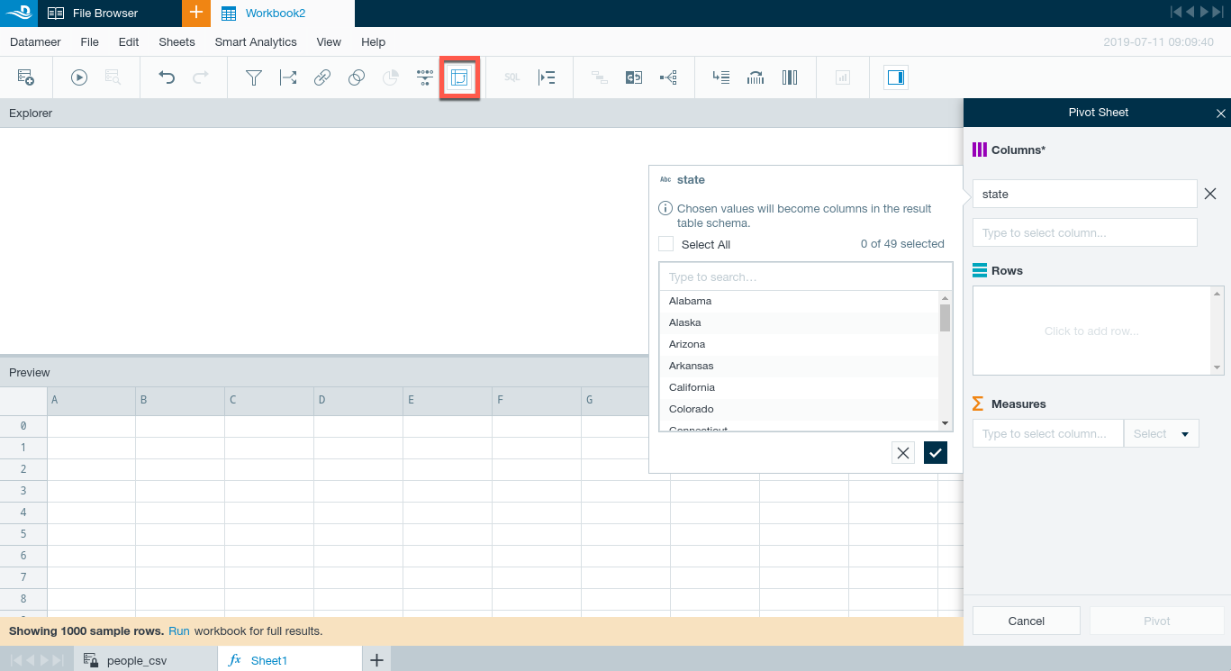
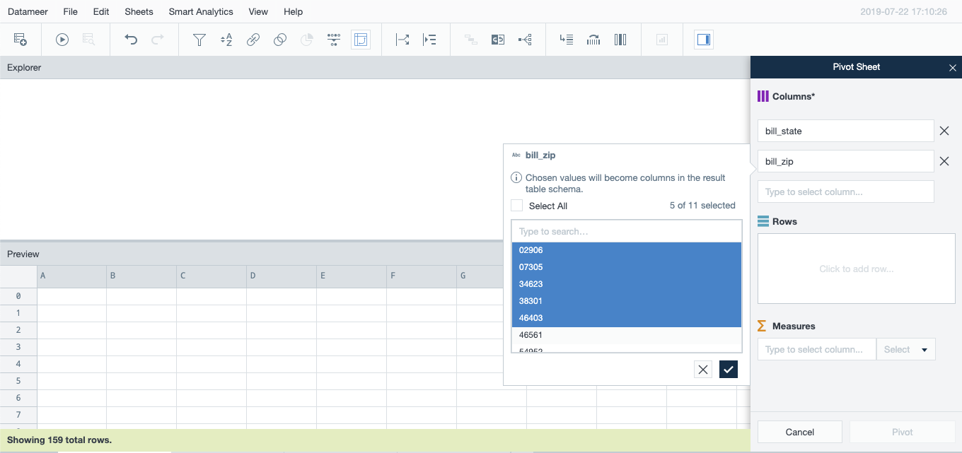
4. Select a column in the first Columns field then click to select the values by which you want to group data. Select All is an option but will not always yield useful results. It is wiser to choose to aggregate by values with lower cardinality so the results will be comprehensible.

   

5. In the Measure fields, select the data characteristics you want to view. Only the columns other than those already selected will be available.

   You must also select an operation. Functions are filtered depending on the data type selected as the measure. FIRST and LAST require an additional OrderBy value.

   

6. Click Pivot to process.

   The Explorer will display the pivot aggregation hierarchically with color coding for columns (purple) and measure (orange).

   The Preview contains the sheet generated by the pivot transformation. The sheet column headers display the actual yielded pivot aggregation and values.

   Note that these panes scroll independently.

7. Once a Pivot sheet is created you can refine the results dynamically by changing values or introducing an additional pivot by Rows.

   The column value you choose in the Rows field becomes a row label in the resulting pivot table. Spitting by rows lets you view and categorize data from an independent angle.

   Typically you would split by rows to view characteristics with fewer values, or to simplify very large datasets with numerous enough values to populate your columns with a high density of results.