Grouping Functions#

In Spectrum grouping functions are split into two distinct types of functions, group series functions and aggregate functions.

Group series functions in Spectrum are similar to aggregation functions - they group values that have the same key, but they don't aggregate values. The biggest difference between group series functions and aggregation functions is that group series functions usually have more than one result per key where as aggregation functions have only one result per key. In order to use these functions you must first define groups within your Workbook. This can be done using the GROUPBY (), GROUPBYBIN (), or GROUPBYGAP () functions.

Group Series Functions#

Group series functions operate row-wise within a group. The function is applied to every row and therefore returns a value for every argument in the group.

INFO

When using a group series function within an IF()'s 2nd or 3rd argument or the functions AND() / OR() in any argument position, Spectrum can't guarantee that all of their arguments will be evaluated.

Problems can occur around lazy evaluation when you are working with the functions that maintain state. This is true for all of the group series functions.

Functions IF, AND, and OR (as well as operators && and ||) arguments are evaluated lazily. This evaluation strategy is used to prevent failures caused by evaluating expressions that may result in an exception.

The following functions in Spectrum are group series functions:

GROUPACCUMULATE#

Syntax#

GROUPACCUMULATE(<number or date>;<number>)

Description#

Returns the sum of all previous records in a group.

This function requires a key column (GROUPBY) and two arguments. The first argument (OrderBy) is the column used for sorting the accumulated values. The second argument (number) is the column of values to be summed within their groups.

This is a group series function and only operates on columns from a data source or join sheet.

Example

Given the following data:

Date	Revenue
Jan 1, 2011	30
Feb 1, 2011	10
Mar 1, 2011	20
Apr 1, 2011	40
May 1, 2011	20
Jun 1, 2011	40
Jul 1, 2011	20
Aug 1, 2011	20
Sep 1, 2011	30
Oct 1, 2011	50
Nov 1, 2011	10
Dec 1, 2011	20
Jan 1, 2012	10
Feb 1, 2012	20
Mar 1, 2012	60
Jan 1, 2013	40
Feb 1, 2013	10
Mar 1, 2013	10

First create a group by the year using GROUPBY(YEAR(#RawData!Date))

Group_Year
2011
2012
2013

Next copy the date column to your group using COPY(#RawData!Date)

Group_Year	Date
2011	Jan 1, 2011
2011	Feb 1, 2011
2011	Mar 1, 2011
2011	Apr 1, 2011
2011	May 1, 2011
2011	Jun 1, 2011
2011	Jul 1, 2011
2011	Aug 1, 2011
2011	Sep 1, 2011
2011	Oct 1, 2011
2011	Nov 1, 2011
2011	Dec 1, 2011
2012	Jan 1, 2012
2012	Feb 1, 2012
2012	Mar 1, 2012
2013	Jan 1, 2013
2013	Feb 1, 2013
2013	Mar 1, 2013

Using GROUPACCUMULATE(#RawData!Date;#RawData!Revenue), Spectrum returns the accumulated sum of all the records within each group.

Group_Year	Date	GROUPACCUMULATE returns
2011	Jan 1, 2011	30
2011	Feb 1, 2011	40
2011	Mar 1, 2011	60
2011	Apr 1, 2011	100
2011	May 1, 2011	120
2011	Jun 1, 2011	160
2011	Jul 1, 2011	180
2011	Aug 1, 2011	200
2011	Sep 1, 2011	230
2011	Oct 1, 2011	280
2011	Nov 1, 2011	290
2011	Dec 1, 2011	310
2012	Jan 1, 2012	10
2012	Feb 1, 2012	30
2012	Mar 1, 2012	90
2013	Jan 1, 2013	40
2013	Feb 1, 2013	50
2013	Mar 1, 2013	60

GROUPBOTTOMN#

Syntax#

GROUPBOTTOMN(<any>;<integer>)

Description#

Selects the bottom N values from a group. If this function is applied on a date column, bottom N means the N least recent dates. This is a group series function.

Example

Given the following data:

Groups	Participants
group1	6
group1	12
group1	5
group1	5
group1	5
group1	7
group1	5
group1	9
group1	8
group2	24
group2	24
group2	24
group2	33
group2	33
group2	29
group2	30
group2	32
group2	35

First create a group using GROUPBY(#RawData!Groups):

Groups
group1
group2

Then use the GROUPBOTTOMN(#RawData!Participants;3), and the result is the bottom "N" (in this case "3") values of the column in relation to the GROUPBY() column.

Groups	Smallest_Participants
group1	5
group1	5
group1	5
group2	24
group2	24
group2	24

GROUPBY#

Syntax#

GROUPBY(<any>)

Description#

This function creates groups based on a key (a column) selected by the user. These groups are then used to sort the results of either aggregate or group series functions. It is possible to create sub-groups by using this function again on another key from the same Workbook sheet. The rows for each group series are highlighted when the GROUPBY function is complete.

Example

Given the following data:

Customer_	Name	Item
2535	Jon	Zamioculcas
2888	Mike	Spider Lily
2535	Jon	Datura
2535	Jon	Dahlia
8654	<null>	Windflower
5788	Jon	Snapdragon
2888	Mike	Marguerite
2535	Jon	Windflower
2888	Mike	Elephant's Ear
2535	Jon	Chinese Evergreen
5788	Jon	Begonia
5788	Jon	Starfish Plant
2535	Jon	Hare's Foot Fern
2535	Jon	Venus Flytrap
3545	Monique	Red Flame Ivy
8654	<null>	Starfish Plant
4587	<null>	Begonia

Use GROUPBY(#RawData!Name) to create initial groups.

Customer
<null>
Jon
Mike
Monique

Use GROUPBY(#RawData!Customer_) to create sub-groups.

Customer	Customer_Number
<null>	4587
<null>	8654
Jon	2535
Jon	5788
Mike	2888
Monique	3545

Use a further group series or aggregation function to look at our results more closely (here use GROUPCOUNT to find the total number of orders per customer).

Customer	Customer_Number	Num_Orders
<null>	4587	1
<null>	8654	2
Jon	2535	7
Jon	5788	3
Mike	2888	3
Monique	3545	1

GROUPBYBIN#

Syntax#

GROUPBYBIN(<numeric>;<integer>)

Description#

This function groups selected values into bins created at a specified size. The second value is the size of the bin.

This is a group series function.

INFO

The GROUPBYBIN argument value can also accept date values though not officially supported and not all date/time parse patterns are available to describe the bin size. Date values are defined by millisecond so that 3,600,000 ms is equal to 1 hour. Simple time/date parse patterns that can be described in milliseconds return correct bin sizes.

Examples:

s = second, m = minute, h = hour, d = day

It isn't possible to create a "month" bin size but is possible to create a bin with a 30 day size.

Example

GROUPBYBIN(<Column1>;<100>)

Column1	Results
456	300
789	400
342	700
419
738

GROUPBYCUSTOMBIN#

Syntax#

GROUPBYCUSTOMBIN(<float>,<integer>;<integer>)

Description#

This function groups selected values into bins created at a custom sizes. In the GROUPBYBIN function only a single bin size can be created. In GROUPBYCUSTOMBIN, you can create multiple bin sizes. This is a group series function.

Example

GROUPBYCUSTOMBIN(<Column1>;10;50;100;500)

In this example, the bin sizes created are 10, 50, 100, and 500. Column1 is the data used in the function to be sorted into bins. The function adds the values from column1 into the defined bins. The GROUPCOUNT function shows the number of values in each bin.

Column1	GROUPBYCUSTOMBIN() result	GROUPCOUNT()
15	10	2
35	50	3
55	100	3
75	500	2
90
122
285
465
578
1028

GROUPBYGAP#

Syntax#

GROUPBYGAP(<number>,<date>;<number>)

Description#

This functions displays values by defined gap sizes from a column. A GROUPBY() function must first be used in order to then find the gaps in arguments of another column in relation to it. When run, the function sorts the numbers or dates in ascending order by group. The results displayed are the data values greater than the user made "max gap" value. These gaps are defined as being from each value to the next subsequent value.

This function can be used for click stream analysis. To do click stream analysis, this function also does a secondary sort on the argument column.

This is a group series function.

INFO

If the first parameter is a date:

A number entered in the second parameter to define the gap will be represented in milliseconds.
A date constant can be used in the second parameter to define the max gap.

Example

The following example extracts sessions from the timestamp column when there is more than a 7 time-unit gap:

Suppose you have this spreadsheet:

User	Timestamp
Ajay	1
Ajay	2
Ajay	3
Ajay	11
Ajay	14
Ajay	21
Mary	2
Mary	4
Mary	6
Mary	11
Mary	21
Daniel	3
Daniel	12
Daniel	9
Daniel	6
Daniel	21
Daniel	18
Daniel	15

First create a group using GROUPBY(\<user>). Then use the GROUPBYGAP(\<timestamp>;7). The result of applying GROUPBYGAP would be:

user	result_timestamp
Ajay	1
Ajay	11
Mary	2
Mary	21
Daniel	3

GROUPCOMBIN#

Syntax#

GROUPCOMBIN(<any>)

Description#

Generates all the unique combinations of the values of a group. The combinations are represented as a list. The combinations must have at least two elements.

This is a group series function. This function returns a list. If you require a JSON represented as a string wrap this function in TOJSON, (e.g., TOJSON(FUNCTION(...)). The maximum amount of rows this function can return is 65,520.

Example

Given the following data:

Column1	Column2
A	1
A	2
A	3
B	1
B	2

Applying the above function results in the following spreadsheet:

Column1	GROUPCOMBIN returns
A	[1,2]
A	[1,2,3]
A	[2,3]
A	[1,3]
B	[1,2]

GROUPPREDICTIVEWINDOWS#

Syntax#

GROUPPREDICTIVEWINDOWS(<string, date, or number>; <string, date, or number>; <string, date, or number>; <date>; <number>)

Description#

This function assigns IDs to events. It does that based on an event that defines the center of a time-based window (center-event) and all events in that window get assigned the ID of the center-event. It returns a two-element list for each event within the window: the timestamp of that event and the ID of the windows center event.

This is a group series function.

Example

Given the following raw data:

Group Name	Event	Date
1	a	Aug 1, 2014
2	b	Aug 2, 2014
3	c	Aug 3, 2014
4	d	Aug 4, 2014
5	e	Aug 5, 2014

Create a new worksheet and use the GROUPBY function with the constant "1" to make a single group.

GROUPBY(1)

Next use the GROUPPREDICTIVEWINDOWS function to create a two-element list for each event within a specified window. The two elements are the date used to create the OrderBy and the Window ID. This example creates a three day window from the specified center event "c" using the value 259200000 milliseconds.

Events = #RawData!Event
Window center event = "c"
Window ID = #RawData!GroupName
OrderBy = #Rawdata!Date
Window size in MS = 259200000

Ensure that values of the string data type are entered with quotation marks.

GROUPPREDICTIVEWINDOWS(#RawData!Event;"c";"#RawData!GroupName;#RawData!Date;259200000)

GROUPBY_Constant	Window
1	[Aug 2, 2014, 3]
1	[Aug 3, 2014, 3]
1	[Aug 4, 2014, 3]

GROUPROWNUMBER#

Syntax#

GROUPROWNUMBER()

Description#

Returns with a created row number for each record in a group series.

This is a group series function.

Example

Given the following data:

	Unit
1	A
2	A
3	A
4	B
5	B
6	C
7	C
8	C
9	C
10	C

First create a group using GROUPBY(#RawData!Unit)

	Unit
1	A
2	B
3	C

Then use the GROUPROWNUMBER(), and the result shows row numbers within a sorted group series in relation to the GROUPBY() column.

	Unit	Row_Number
1	A	1
2	A	2
3	A	3
4	B	1
5	B	2
6	C	1
7	C	2
8	C	3
9	C	4
10	C	5

GROUPSESSIONS#

Syntax#

GROUPSESSIONS(<string, date, or number>; <string, date, or number>; >; <string, date, or number>; <string, date, or number>)

Description#

Assigns IDs to events based on session start and session end. All events with the session ID of the start event between start and end event get assigned the ID of the start event.

This is a group series function.

Example

Given the following raw data:

GroupName	Event	Date
1	A	Aug 1, 2014
1	B	Aug 2, 2014
2	start	Aug 3, 2014
2	A	Aug 4, 2014
2	A	Aug 5, 2014
2	end	Aug 6, 2014
3	B	Aug 7, 2014
3	start	Aug 8, 2014
3	end	Aug 9, 2014
3	A	Aug 10, 2014

Create a new worksheet and use the GROUPBY function to group by the GroupName column from the raw data.

GROUPBY(#rawdata!GroupName)

COPY the event and date columns for reference.

COPY(#rawdata!Event)
COPY(#rawdata!Date)

GroupName	Event	Date
1	A	Aug 1, 2014
1	B	Aug 2, 2014
2	start	Aug 3, 2014
2	A	Aug 4, 2014
2	A	Aug 5, 2014
2	end	Aug 6, 2014
3	B	Aug 7, 2014
3	start	Aug 8, 2014
3	end	Aug 9, 2014
3	A	Aug 10, 2014

Use the GROUPSESSIONS function to create a column that assigns a session ID for each event with the same session ID of the "start" marker between the "start" and "end" markers.

Events = #rawdata!Event
Start event = "start"
End event = "end"
Session ID = #rawdata!GroupName
OrderBy =   #rawdata!Date

Ensure that values of the string data type are entered with quotation marks.

GROUPSESSIONS(#rawdata!Event;"start";"end";#rawdata!GroupName;#rawdata!Date)

GroupName	Event	Date	SessionId
1	A	Aug 1, 2014	\
1	B	Aug 2, 2014	\
2	start	Aug 3, 2014	2
2	A	Aug 4, 2014	2
2	A	Aug 5, 2014	2
2	end	Aug 6, 2014	2
3	A	Aug 10, 2014	\
3	B	Aug 7, 2014	\
3	start	Aug 8, 2014	3
3	end	Aug 9, 2014	3

GROUPTOPN#

Syntax #

GROUPTOPN(<any>;[<integer>])

Description#

Selects the top N values from a group. If this function is applied on a date column, top N means the N most recent dates.

This is a group series function.

Example

Given the following data:

Groups	Participants
group1	6
group1	12
group1	5
group1	5
group1	5
group1	7
group1	5
group1	9
group1	8
group2	24
group2	24
group2	24
group2	33
group2	33
group2	29
group2	30
group2	32
group2	35

First create a group using GROUPBY(#RawData!Groups)

Groups
group1
group2

Then use the GROUPTOPN(#RawData!Participants;3). The result is the top "N" (in this case "3") values of the column in relation to the GROUPBY() column.

Groups	Participants_TOP3
group1	12
group1	9
group1	8
group2	35
group2	33
group2	33

GROUPUNIQUES#

Syntax#

GROUPUNIQUES(<any>)

Description#

Returns unique column values for a group.

This is a group series function.

Example

Given the following raw data:

Key	Value
1	0
1	1
2	1
1	0
1	2
2	1
2	1
2	0
2	1
1	1
2	\
1	a

Create a new worksheet and use the GROUPBY function to group by the Key column from the raw data.

GROUPBY(#RawData!Key)

Next use the GROUPUNIQUES function to create a column which returns the unique values of each group.

GROUPUNIQUES(#RawData!Value)

Key_Groups	Unique_Value
1	0
1	1
1	2
1	a
2	\
2	0
2	1

GROUP_DIFF#

Syntax#

GROUP_DIFF(<number or date>; [<number>])

Description#

Calculates the difference between the current value and the previous value seen in the group. The optional ["initial value"] argument is used as result for the first record. This defaults to null.

This is a group series function.

Example

Given the following data:

Groups	Participants
group1	6
group1	12
group1	5
group1	5
group1	5
group1	7
group1	5
group1	9
group1	8
group2	24
group2	24
group2	24
group2	33
group2	33
group2	29
group2	30
group2	32
group2	35

First create a group, e.g. GROUPBY(#RawData!Groups)

Groups
group1
group2

Then use the GROUP_DIFF(#RawData!Participants), and the results show the difference between the current value the previous value in relation to the GROUPBY() column.

Groups	Participants_DIFF
groups1	<null>
groups1	6
groups1	-7
groups1	0
groups1	0
groups1	2
groups1	-2
groups1	4
groups1	-1
groups2	<null>
groups2	0
groups2	0
groups2	9
groups2	0
groups2	-4
groups2	1
groups2	2
groups2	3

Example 2

The following example illustrates how to compute the time a user has spent on a web site.

=GROUPBY(#Sheet1!session)
=GROUP_SORT_ASC(#Sheet1!timestamp)
=GROUP_PATH(#Sheet1!url)
=GROUP_DIFF(#Sheet1!timestamp)

Suppose we have this spreadsheet:

session	timestamp	url
session1	20	url1
session1	25	url2
session2	40	url1
session1	55	url3

The result sheet looks like this:

session	timestamp	click_path	time_spent
session1	20	["external":"url1"]	\
session1	25	["url1":"url2"]	5
session1	55	["url2":"url3"]	30
session1	55	["url3":"external"]	\
session2	40	["external":"url1"]	\
session2	40	["url1":"external"]	\

Note that the first value for a group in the time_spent column is empty, because there is no real time spent before you make the first request to the web server. You could use any other default by setting the second argument of GROUP_DIFF, e.g. GROUP_DIFF(#Sheet1!timestamp; 0). There are also empty (or null) values in this column for the last record of a group, because there is no time_spent that could be computed when leaving a web page. Leaving a web page is determined when there are no further requests, but you have no idea how long somebody spent on the last page he or she visits.

If you were to use GROUP_DIFF on two times stamps that use the second granularity, results are returned in milliseconds.

The sorting function GROUP_SORT_ASC is being used on the same sheet as where it is later being referenced by the function GROUP_DIFF. Insure the column being sorted is on the sheet where it is being referenced.

GROUP_PAIR#

Syntax#

GROUP_PAIR(<any>)

Description#

Generates all unique pairs of the values of a group. These pairs are returned as a list.

This is a group series function.

Example

Given the following data:

Groups	Items
group1	apple
group1	banana
group1	pear
group2	apple
group2	banana
group2	apple
group3	apple

First create a group using GROUPBY(#RawData!Groups)

Groups
group1
group2
group3

Then use the GROUP_PAIR(#RawData!Items). The results are all the combinations of possible pairs of the column represented as a list in relation to the GROUPBY() column.

Groups	Item_PAIR
group1	["apple","banana"]
group1	["banana","pear"]
group1	["apple","pear"]
group2	["apple","banana"]

This function returns a list. If you require a JSON represented as a string, wrap this function in TOJSON (E.g., TOJSON(<function>(...)).

GROUP_PATH#

Syntax#

GROUP_PATH(<any>)

Description#

Displays the path from one point to another for all values in a group. This can be used for click stream analysis.

This is a group series function.

Also see:

GROUP_PATH_CHANGES To filter out paths where the URL doesn't change.
GROUPBYGAP To extract sessions from gaps in a timestamp.

Example

This example is a simple click stream analysis that displays the path during specified sessions.

Given the following data:

session	timestamp	url
session1	2	url1
session1	3	url1
session1	4	url2
session2	5	url1
session2	6	url2
session1	7	url3
session2	8	url1
session1	9	url2
session2	10	url1

First create a group using GROUPBY(#RawData!session).

session
session1
session2

Next sort your timestamp in ascending order using GROUP_SORT_ASC(#RawData!timestamp).

session	timestamp
session1	2
session1	3
session1	4
session1	7
session1	9
session2	5
session2	6
session2	8
session2	10

Then use the GROUP_PATH(#RawData!url). The result shows paths for all values of the column in ascending order in relation to the GROUPBY() column.

session	timestamp	url_Path
session1	2	["external","url1"]
session1	3	["url1","url1"]
session1	4	["url1","url2"]
session1	7	["url2","url3"]
session1	9	["url3","url2"]
session1	9	["url2","external"]
session2	5	["external","url1"]
session2	6	["url1","url2"]
session2	8	["url2","url1"]
session2	10	["url1","url1"]
session2	10	["url1","external"]

GROUP_PATH_CHANGES#

Syntax#

GROUP_PATH_CHANGES(<any>)

Description#

Create paths from a field, but only if the value changes. This function can be used for click stream analysis.

This is a group series function.

Also see:

GROUP_PATH To not filter out paths where the URL doesn't change.
GROUPBYGAP To extract sessions from gaps in a timestamp.

Example

Analyze click streams, group on a session, sort by timestamp, and generate the clicks paths.

Given the following data:

session	timestamp	url
session1	2	url1
session1	3	url1
session1	4	url2
session2	5	url1
session2	6	url2
session1	7	url3
session2	8	url1
session1	9	url2
session2	10	url1

First create a group using GROUPBY(#RawData!session).

session
session1
session2

Next, sort your timestamp in ascending order using GROUP_SORT_ASC(#RawData!TimeStamp).

sessions	Ascending_TimeStamp
session1	2
session1	3
session1	4
session1	7
session1	9
session2	5
session2	6
session2	8
session2	10

Then use the GROUP_PATH(#RawData!url). The result shows paths for values that have changed in the column, in ascending order, in relation to the GROUPBY() column.

Sessions	Ascending_TimeStamp	url_PATH_CHANGE
session1	2	["external","url1"]
session1	4	["url1","url2"]
session1	7	["url2","url3"]
session1	9	["url3","url2"]
session1	9	["url2","external"]
session2	5	["external","url1"]
session2	6	["url1","url2"]
session2	8	["url2","url1"]
session2	10	["url1","external"]

GROUP_PREVIOUS#

Syntax#

GROUP_PREVIOUS(<any>;[<number>])

Value: series value

K: lag

Description#

Returns the value of the set k'th previous record in series. This can be used for introducing a lag for time series analysis and/or computing autocorrelation.

This is a group series function.

Example

Given the following data:

Groups	Number
group1	4
group1	5
group1	6
group2	7
group2	8
group1	9
group1	10
group2	11
group2	12
group1	13
group2	14
group1	15

First create a group using GROUPBY(#RawData!Groups).

Groups
group1
group2

Then use the GROUP_PREVIOUS(#RawData!Number). The result shows the previous record's value in relation to the GROUPBY() column.

Groups	PREVIOUS_Number
group1	<null>
group1	4
group1	5
group1	6
group1	9
group1	10
group1	13
group1	15
group2	<null>
group2	7
group2	8
group2	11
group2	12
group2	14

Example 2

The following example illustrates how to compute the time a user has spent on a web site.

Given the following data:

Session	TimeStamp	url
session1	20	url1
session1	25	url2
session2	40	url1
session1	55	url3

First create a group using GROUPBY(#RawData!Session).

Session
session1
session2

In order for the GROUP_PREVIOUS function to work, you need to use GROUP_SORT_ASC in conjunction. Sorting data isn't sufficient.

Next sort your timestamp in ascending order using GROUP_SORT_ASC(#RawData!TimeStamp)

Session	Ascending_TimeStamp
session1	20
session1	25
session1	55
session2	40

Next use the GROUP_PATH(#RawData!url). The result shows paths for all values of the column in ascending order in relation to the GROUPBY() column.

Session	Ascending_TimeStamp	url_PATH
session1	20	["external","url1"]
session1	25	["url1","url2"]
session1	55	["url2","url3"]
session1	55	["url3","external"]
session2	40	["external","url1"]
session2	40	["url1","external"]

Next use GROUP_PREVIOUS(#RawData!TimeStamp)

Session	Ascending_TimeStamp	url_PATH	Previous_TimeStamp
session1	20	["external","url1"]	<null>
session1	25	["url1","url2"]	20
session1	55	["url2","url3"]	25
session1	55	["url3","external"]	55
session2	40	["external","url1"]	<null>
session2	40	["url1","external"]	40

Finally use DIFF(#Sheet1!Ascending_TimeStamp;#Sheet1!Previous_TimeStamp) to subtract the ascending TimeStamp from the Previous_TimeStamp to find how long the user spend on the URL.

Session	Ascending_TimeStamp	url_PATH	Previous_TimeStamp	Time_Spent
session1	20	["external","url1"]	<null>	20
session1	25	["url1","url2"]	20	5
session1	55	["url2","url3"]	25	30
session1	55	["url3","external"]	55	0
session2	40	["external","url1"]	<null>	40
session2	40	["url1","external"]	40	0

GROUP_SORT_ASC#

Syntax#

GROUP_SORT_ASC(<any>)

Description#

Sorts groups in ascending order.

This is a group series function.

The sort results can't be guaranteed to transfer from one sheet to another due to the nature of distributed systems. Ensure the sort was made on the sheet where it is being referenced.

Example

Given the following data:

Group	Users
group1	5
group1	8
group2	9
group1	7
group1	9
group2	12
group2	10
group2	4
group1	2
group1	6

First create a group using GROUPBY(#RawData!Group).

Group
group1
group2

Then use the GROUP_SORT_ASC(#RawData!Users). The result is the column values displayed in ascending order in relation to the GROUPBY() column.

Group	Ascending_Users
group1	2
group1	5
group1	6
group1	7
group1	8
group1	9
group2	4
group2	9
group2	10
group2	12

GROUP_SORT_DESC#

Syntax#

GROUP_SORT_DESC(<any>)

Description#

Sorts groups in descending order. This can be used for click stream analysis.

This is a group series function.

The sort results can't be guaranteed to transfer from one sheet to another due to the nature of distributed systems. Ensure the sort was made on the sheet where it is being referenced.

Example

Given the following data:

Group	Users
group1	5
group1	8
group2	9
group1	7
group1	9
group2	12
group2	10
group2	4
group1	2
group1	6

First create a group using GROUPBY(#RawData!Group).

Group
group1
group2

Then use the GROUP_SORT_DESC(#RawData!Users). The result is the column values displayed in descending order in relation to the GROUPBY() column.

Group	Decending_Users
group1	9
group1	8
group1	7
group1	6
group1	5
group1	2
group2	12
group2	10
group2	9
group2	4

Aggregate Functions#

Aggregate functions combine and then operate on all the values in a group. The function returns one value for each group.

INFO

Due to the different nature of group series functions and aggregate functions, they can't be used in the same Workbook sheet.

INFO

Aggregations functions applied to empty groups (all records have been filtered) will result in no entry, e.g. GROUPCOUNT() will not return 0 but no record.

The following functions in Spectrum are aggregate functions:

GROUPAND#

Syntax#

GROUPAND(<boolean>)

Description#

This function checks if all arguments are true for an entire column of Boolean values that has been grouped with the GROUPBY() function.

The function returns true if all arguments are true. The function returns false if any of the arguments are false.

Example

Given the following data:

Group	User	Login
1	adam	true
1	bob	true
2	chris	true
2	dave	false
2	eric	false

First create a group, e.g. GROUPBY(#RawData!group)

GroupBy
1
2

Then use the GROUPAND(#RawData!login), and the results are a Boolean value based on the AND() function of your grouped data.

GroupBy	Group_And returns
1	true
2	false

GROUPANOVA#

Syntax#

GROUPANOVA(<string>|<integer>,<integer>|<float>;<float>)

Description#

This function is for comparing the means of three or more samples to see if they are significantly different at a certain significance level (usually alpha=0.05).

A JSON object is returned with the calculated F-statistic, the degrees of freedom between the groups, the degrees of freedom with in the groups, the P-value, and a statement if the difference is significant or not.

The function arguments are: - Sample ID column - Value column - Significance level constant (optional)

Example

Example input sheet:

Experiment	Sample_ID	Value
A	x	12
A	x	15
A	x	9
A	y	20
A	y	19
A	y	23
A	z	40
A	z	35
A	z	42

Using GROUPBY(#input!Experiment) and GROUPANOVA(#input!Sample_ID;#input!value;0.05)

Experiment	GROUPANOVA returns
A	{"f-statistic":64.95,"dfbg":2,"dfwg":6,"isSignificant":true}

GROUPANY#

Syntax#

GROUPANY(<any>)

Description#

Returns an arbitrarily selected value contained in the group. The selection process is not completely random, but you can't influence which value is selected. This function used to be called GROUPFIRST and has been renamed GROUPANY in version 1.4.

Example

Given the following data:

Customer	Name	Item
2535	Jon	Zamioculcas
2888	Mike	Spider Lily
2535	Jon	Datura
2535	Jon	Dahlia
5788	Jon	Snapdragon
2888	Mike	Marguerite
2535	Jon	Windflower
2888	Mike	Elephant's Ear
2535	Jon	Chinese Evergreen
5788	Jon	Begonia
5788	Jon	Starfish Plant
2535	Jon	Hare's Foot Fern
2535	Jon	Venus Flytrap
3545	Monique	Red Flame Ivy

First create a group e.g. GROUPBY(#RawData!Customer_).

Customer
2535
2888
3545
5788

Then use GROUPANY(#RawData!Item), and an arbitrary value from that column appears.

Customer	GROUPANY returns
2535	Zamioculcas
2888	Spider Lily
3545	Red Flame Ivy
75788	Snapdragon

GROUPAVERAGE#

Syntax#

GROUPAVERAGE(<number>)

Description#

Returns the average value of a group by creating a sum for all values in the group and dividing by the number of values. A GROUPBY() function must first be used in order to then find the average arguments of another column in relation to it. The value of the GROUPAVERAGE() must be a number and is returned as a float.

Empty or <null> records of a group aren't calculated into GROUPAVERAGE().

Calculating a column with a (or multiple) <error> records always returns an error for its group.

Example

Given the following data set:

user_screen_name	user_follower_count	user_friend_count	user_time_zone
ArteWorks_SEO	2605	345	Central Time (US & Canada)
evan_b	460	316	Pacific Time (US & Canada)
briancoffee	185	321	London
PhillisGene	280	<null>	London
SsReyes	4	4	Pacific Time (US & Canada)
addztickets	291	0	Central Time (US & Canada)
mynossseee	190	94	Melbourne
AprilBraswell	14206	14082	Pacific Time (US & Canada)
bebacklatersoon	234	103	Sydney
nicolebaker76	7	3	London
Object5	512	<error>	Melbourne
tman2088	108	155	Central Time (US & Canada)

First create a group, e.g. GROUPBY(#RawData!user_time_zone)

user_time_zone
Alaska
Central Time (US & Canada)
London
Melbourne
Pacific Time (US & Canada)
Sydney

Then use the GROUPAVERAGE(#RawData!user_friends_count), and the average value of the arguments of that column appears in relation to the GROUPBY() column.

user_time_zone	GROUPAVERAGE returns
Alaska	27
Central Time (US & Canada)	166.6666667
London	162
Melbourne	<error>
Pacific Time (US & Canada)	4800.666667
Sydney	27

GROUPCONCAT#

Syntax#

GROUPCONCAT(<any>;[<any>])

Description#

Creates a list of all unique non-null values seen in a group (currently max. 1000 values are collected). The order of elements isn't stable when running on a cluster, because the elements for each group might be collected on different nodes. If the element order matters, provide an order by expression as a second (optional) argument. This could for example be a timestamp or ID column in your data set.

INFO

This function returns a list. If you require a JSON represented as a string wrap this function in TOJSON (E.g., TOJSON((...)).

Example

Given the following data:

Key	Value	Time_Stamp
group1	a	1
group1	b	4
group1	c	3
group1	d	2
group2	a	4
group2	b	3
group2	c	2
group2	d	1

First create a group, e.g. !GROUPBY(#RawData!Key)

Groups
group1
group2

Then use the !GROUPCONCAT(#RawData!Value;#RawData!Time_Stamp), and the result is a list ordered by the identifier in relation to the GROUPBY() column.

Groups	Value
group1	[a, d, c, b]
group2	[d, c, b, a]

GROUPCONCATDISTINCT#

Syntax#

GROUPCONCATDISTINCT(<any>;[<number>])

Description#

Concatenates all non-null values seen in a group. The first argument is the column containing values that should be concatenated. The second value is an optional constant used to set a maximum number of values to avoid overflow problems with very large groups. The maximum number of values defaults to 1000. If more than the configured maximum number n of values are seen, the top n values in ascending order are kept.

The concatenated values are returned as a list.

INFO

This function returns a list. If you require a JSON represented as a string, wrap this function in TOJSON (E.g., TOJSON((...)).

Example

Given the following data:

Groups	Items
group1	2
group1	5
group1	<null>
group1	17
group1	8
group2	<null>
group2	6
group2	6
group2	5
group2	12
group3	<null>
group3	<null>
group3	22
group3	25
group3	12

First create a group using GROUPBY(#RawData!Groups)

Groups
group1
group2
group3

Then use the GROUPCONCATDISTINCT(#RawData!Items;2) and the result is the non-null values concatenated in the number of groups you specified by the constant.

Groups	Item_CONCAT
group1	[2, 5]
group2	[5, 6]
group3	[12, 22]

GROUPCOUNT#

Syntax#

GROUPCOUNT()

Description#

Counts the records in one group. No calculations are performed with this function. Empty or records of a group are calculated into GROUPCOUNT().

The GROUPCOUNT function results in an error only if the grouping itself contains an error.

Example

Given the following data:

Customer_	Name	Item
2535	Jon	Zamioculcas
2888	Mike	Spider Lily
2535	Jon	Datura
2535	Jon	Dahlia
8654		Windflower
5788	Jon	Snapdragon
2888	Mike	Marguerite
2535	Jon	Windflower
2888	Mike	Elephant's Ear
2535	Jon	Chinese Evergreen
5788	Jon	Begonia
5788	Jon	Starfish Plant
2535	Jon	Hare's Foot Fern
2535	Jon	Venus Flytrap
3545	Monique	Red Flame Ivy
8654		Starfish Plant
4587		Begonia
1234	<error>	Elephant's Ear
4321	<error>	Snapdragon

First create a group using GROUPBY(#RawData!Name)

Name
<error>

Jon
Mike
Monique

Use !GROUPCOUNT() to return the amount of times a given argument appears, in relation to the GROUPBY() column.

Name	-
<error>	<error>
\	3
Jon	10
Mike	3
Monique	1

GROUPCOUNTDISTINCT#

Syntax#

GROUPCOUNTDISTINCT(<any>)

Description#

Counts the distinct values of a group.

Out of Memory

Known Issue - When working with the GROUPCOUNTDISTINCT function on a dataset with a very high number of records in a group, out of memory exceptions might occur.
Cause - In order to determine the true distinct value, GROUPCOUNTDISTINCT shifts all mapped information to disk on one reducer. This can cause disk space and performance/memory issues on large datasets. This is a known limitation that Spectrum is working to resolve.
Solution - In order to work around this issue, an intermediary sheet along with a combination of GROUPBY and GROUPCOUNT functions is suggested as described below.

Original

Sheet 1: user_id, product
Sheet 2: GROUPBY(Sheet1.product), GROUPCOUNTDISTINCT(Sheet2.user_id)

Workaround:

Sheet 1: user_id, produt
Sheet 2: groupby(Sheet1.product), groupby(Sheet1.user_id)
Sheet 3: group by(Sheet2.product), groupcount

This workaround gives the same desired output of the GROUPCOUNTDISTINCT function.

Example

Given the following data:

Customer_	Name	Item
2535	Jon	Zamioculcas
2888	Mike	Spider Lily
2535	Jon	Datura
2535	Jon	Dahlia
5788	Jon	Snapdragon
2888	Mike	Marguerite
2535	Jon	Windflower
2888	Mike	Elephant's Ear
2535	Jon	Chinese Evergreen
5788	Jon	Begonia
5788	Jon	Starfish Plant
2535	Jon	Hare's Foot Fern
2535	Jon	Venus Flytrap
3545	Monique	Red Flame Ivy

First create a group using (#RawData!Name)

Name
Jon
Mike
Monique

Then use the !GROUPCOUNTDISTINCT(#RawData!Customer_), and the results are a count of each time an individual value appears in that column in relation to the GROUPBY() column.

Name	Customer_COUNTDISTINCT
Jon	2
Mike	1
Monique	1

GROUPFIRST#

Syntax#

GROUPFIRST(<any>;order by any)

Description#

This function returns a value in a group as specified by the ordered column's first value.

If the column used to order the group is a number, then the value used from the order column is the lowest number.
If the column used to order the group is a string, then the value used from the order column is the lowest number (in string form). If no numbers (in string form) are present, the first capital letter alphabetically is used. If no uppercase letters are present, the first lowercase letter alphabetically is used.
If the column used to order the group is a date, then the value used from the order column is the earliest date.

Example

Given the following raw data:

Customer_number	Name	Order_number	Item
2535	Jon	101544	Zamioculcas
2888	Mike	101567	Spider Lily
2535	Jon	101643	Datura
2535	Jon	101899	Dahlia
5788	Jon	102003	Snapdragon
2888	Mike	102248	Marguerite
2535	Jon	102282	Windflower
2888	Mike	102534	Elephant's Ear
2535	Jon	102612	Chinese Evergreen
5788	Jon	102617	Begonia
5788	Jon	102765	Starfish Plant
2535	Jon	102947	Hare's Foot Fern
2535	Jon	103001	Venus Flytrap
3545	Monique	103006	Red Flame Ivy

Create a group, using GROUPBY(#RawData!Customer_number), and GROUPBY(#RawData!Name).

Customer_number	Name
2535	Jon
2888	Mike
3545	Monique
5788	Jon

Using GROUPFIRST(#RawData!Item;#RawData!Order_number), you can return the first item ordered by each customer.

Customer_number	Name	First_Item
2535	Jon	Zamioculcas
2888	Mike	Spider Lily
3545	Monique	Red Flame Ivy
5788	Jon	Snapdragon

GROUPJSONOBJECTMERGE#

Syntax#

GROUPJSONOBJECTMERGE()

Description#

Merges all elements in a grouped series of JSON maps.

When JSON Objects with the same key are merged, the earlier key value(s) are overwritten by the following key value(s) in the group.

Example

Given the following data:

Group	Map
Group1	{"Andy":"Sales","Alba":Development","Anna":"Marketing","Affa":Management"}
Group1	{"Jeff":"Sales","June":"Sales","Jack":"Development"}
Group2	{"Sales":"Auto","Development":Auto","Marketing":"Hardware","Management":Auto"}
Group2	{"Sales":"Hardware","Sales":Hardware","Development":"Hardware"}

First create a group using GROUPBY(#RawData!Groups)

GroupBy_Groups
Group1
Group2

Then use GROUPJSONOBJECTMERGE(#Sheet1!Map), and the results are the elements of the groups series merged by key.

GroupBy_Groups	Group_Json_Object_Merge
Group1	{"Andy":"Sales","Alba":Development","Anna":"Marketing","Affa":Management","Jeff":"Sales","June":"Sales","Jack":"Development"}
Group2	{"Sales":"Hardware","Development":Hardware","Marketing":"Hardware","Management":"Auto"}

GROUPLAST#

Syntax#

GROUPLAST(<any>; order by any)

Description#

This function returns a value in a group as specified by the ordered column's last value.

If the column used to order the group is a number, then the value used from the order column is the highest number.
If the column used to order the group is a string, then the value used from the order column is a lowercase letter starting with z and moving reverse alphabetically followed by uppercase letters reverse alphabetically. If no letters are present in the sting type, the value used is the highest number.
If the column used to order the group is a date, then the value used from the order column is the latest date.

Example

Given the following data:

Customer_	Name	Order	Item
2535	Jon	101544	Zamioculcas
2888	Mike	101567	Spider Lily
2535	Jon	101643	Datura
2535	Jon	101899	Dahlia
5788	Jon	102003	Snapdragon
2888	Mike	102248	Marguerite
2535	Jon	102282	Windflower
2888	Mike	102534	Elephant's Ear
2535	Jon	102612	Chinese Evergreen
5788	Jon	102617	Begonia
5788	Jon	102765	Starfish Plant
2535	Jon	102947	Hare's Foot Fern
2535	Jon	103001	Venus Flytrap
3545	Monique	103006	Red Flame Ivy

First create a group using GROUPBY(#RawData!Customer_), and GROUPBY(#RawData!Name).

Customer_	Name
2535	Jon
2888	Mike
3545	Monique
5788	Jon

Using GROUPLAST(#RawData!Item;#RawData!Order), you can return the last item ordered by each customer.

Customer_	Name	Last_Item
2535	Jon	Venus Flytrap
2888	Mike	Elephant's Ear
3545	Monique	Red Flame Ivy
5788	Jon	Starfish Plant

GROUPMAP#

Syntax#

GROUPMAP(<any>; <any>)

Description#

Creates a JSON map based on two columns of all records within a group, keys, and values.

Example

Given the following data:

Customer_	Name	Item
2535	Jon	Zamioculcas
2888	Mike	Spider Lily
2535	Jon	Datura
2535	Jon	Dahlia
5788	Jon	Snapdragon
2888	Mike	Marguerite
2535	Jon	Windflower
2888	Mike	Elephant's Ear
2535	Jon	Chinese Evergreen
5788	Jon	Begonia
5788	Jon	Starfish Plant
2535	Jon	Hare's Foot Fern
2535	Jon	Venus Flytrap
3545	Monique	Red Flame Ivy

First create a group using GROUPBY(#RawData!Name)

Name
Jon
Mike
Monique

Then use the GROUPMAP(#RawData!Item;#RawData!Customer_), and the result is a JSON map based on your two column records in relation to the GROUPBY() column.

Name	\
Jon	{"Zamioculas":2535,"Datura":2535,"Dahlia":2535,"Snapdragon":5788,"Windflower":2535,"Chinese Evergreen":2535,"Begonia":5788,"Starfish Plant":5788,"Hare's Foot Fern":2535,"Venus Flytrap":2535}
Mike	{"Spider Lily":2888,"Maguerite":2888,"Elephant's Ear":2888}
Monique	{"Red Flame Ivy":3545}

GROUPMAX#

Syntax#

GROUPMAX(<number>)

Description#

Returns the maximum values in a group. A GROUPBY() function must first be used in order to then find the maximum arguments of another column in relation to it.

Example

Given the following data:

Name	Number
Ajay	27087
Ajay	55317
Alice	14489
Ajay	31310
Ajay	57822
Ajay	63855
Alice	47640
Alice	48979

First create a group using GROUPBY(#RawData!Name).

Name
Ajay
Alice

Then use GROUPMAX(#RawData!Number) to return the maximum values of the Number column.

Name	Max_Number
Ajay	63855
Alice	48979

GROUPMEDIAN#

Syntax#

GROUPMEDIAN(<number>)

Description#

Returns the medium of all values in a group.

Example

Given the following data:

Groups	Participants
group1	6
group1	12
group1	5
group1	5
group1	5
group1	7
group1	5
group1	9
group1	8
group2	24
group2	24
group2	24
group2	33
group2	33
group2	29
group2	30
group2	32
group2	35

First create a group using GROUPBY(#RawData!Groups)

Groups
group1
group2

Then use the GROUPMEDIAN(#RawData!Participants), and the result is the medium number of the column in relation to the GROUPBY() column.

Groups	Participants_MEDIAN
group1	6
group2	30

GROUPMIN#

Syntax#

GROUPMIN(<number>)

Description#

Returns the minimum values in a group. A GROUPBY() function must first be used in order to then find the minimum arguments of another column in relation to it.

Example

Given the following data:

Name	Number
Ajay	27087
Ajay	55317
Alice	14489
Ajay	31310
Ajay	57822
Ajay	63855
Alice	47640
Alice	48979

First create a group using GROUPBY(#RawData!Name).

Name
Ajay
Alice

Then use GROUPMIN(#RawData!Number) to return the minimum values of the Number column.

Name	Min_Number
Ajay	27087
Alice	14489

GROUPOR#

Syntax#

GROUPAND(<boolean>)

Description#

This function checks if any arguments are true for an entire column of Boolean values that has been grouped with the GROUPBY() function.

The function returns true if any of the arguments are true.

The function returns false if all of the arguments are false.

Example

Given the following data:

group	user	login
1	adam	true
1	bob	true
2	chris	true
2	dave	false
2	eric	false

First create a group using GROUPBY(#RawData!group)

GroupBy
1
2

Then use the GROUPOR(#RawData!login), and the results is a Boolean value based on the OR() function of your grouped data.

GroupBy	Group_Or
1	true
2	true

GROUPPERCENTILE#

Syntax#

GROUPPERCENTILE(<number>; [<number>])

Description#

Return the number which is nth percentile in this distribution as float. The value returned by this function identifies the point where N% of the samples of the distribution are smaller than the Nth percentile. The first argument is the data column, the second argument is N (a value between 0 and 100).

This function calculates this value by first counting the total number of values in the group and using the nth percent of that as a positioning value. Finally, the function orders all values from lowest to highest, and returns the value that is in the position calculated earlier.

The position is calculated using the following formula:

Position = ((N/100) * (number of values -1)) +1

The percentile is then calculated using the following formula if the position isn't a whole number:

Percentile = value of rounded down position + the decimal value of the position * (value of rounded up position - value of rounded down position)

Example

Given the following data:

Groups	Participants
group1	6
group1	12
group1	5
group1	5
group1	5
group1	7
group1	5
group1	9
group1	8
group2	24
group2	24
group2	24
group2	33
group2	33
group2	29
group2	30
group2	32
group2	35

First create a group using GROUPBY(#RawData!Groups). This groups the values of group1 and group2 together in order to figure out the percentile.

Groups
group1
group2

Then use the GROUPPERCENTILE(#RawData!Participants;80) function, and the result is a float that is the nth percentile (in this case 80th percentile) in relation to the GROUPBY() column. In this example, the function calculates the value at which 80 percent of the values in the data column are below that number and 20 percent of the values in that data column are above.

Groups	Participants_PERCENTILE
group1	8.4
group2	33

For example, group1's percentile is calculated by first counting the number of values, which is 9, which then calculates position value using the positioning formula:

Position(80%) = (80/100 * 9 - 1) + 1 = 7.4

The resulting number, 7.4, is used as a placement marker. All of the values are arranged in order from lowest to highest (5,5,5,5,6,7,8,9,12), and GROUPPERCENTILE returns the value that is in the 7.4th position using the percentile formula:

Percentile(7.4) = 8 + 0.4 * (9 - 8) = 8.4

GROUPSELECT#

Syntax#

GROUPSELECT(<any>;<any>;<any>)

Description#

Create columns with selected values using a key constant from a specified grouped column in the Workbook.

Select a column from a worksheet and write in a constant from that column. Next, select the value column for which to compare the constant from the original column. The column being selected isn't allowed to contain different values for the key constant. If there are different values for a key constant, an error results.

This is a excellent tool to create columns for use in a pivot table.

Example

Original Data:

Department	Year	Dollar
Department 1	2010	10
Department 1	2010	20
Department 1	2011	10
Department 2	2011	10
Department 2	2012	10
Department 1	2013	30
Department 1	2013	30
Department 2	2013	35

Create a new worksheet:

GROUPBY(#RawData!Department)
GROUPSELECT(#RawData!Year;2010;#RawData!Dollar)
GROUPSELECT(#RawData!Year;2011;#RawData!Dollar)
GROUPSELECT(#RawData!Year;2012;#RawData!Dollar)
GROUPSELECT(#RawData!Year;2013;#RawData!Dollar)

Department	Dollar_in_2010	Dollar_in_2011	Dollar_in_2012	Dollar_in_2013
Department 1	<error>	10	<empty>	30
Department 2	\	10	10	35

GROUPSTDEVP#

Syntax#

GROUPSTDEVP(<number>)

Description#

Estimates standard deviation on the entire population. If they represent only a sample of the entire population, use GROUPSTDEVS instead.

Example

Given the following data:

Groups	Participants
group1	6
group1	12
group1	5
group1	5
group1	5
group1	7
group1	5
group1	9
group1	8
group2	24
group2	24
group2	24
group2	33
group2	33
group2	29
group2	30
group2	32
group2	35

First create a group using GROUPBY(#RawData!Groups)

Groups
group1
group2

Then use the GROUPSTDEVP(#RawData!Participants), and the result is a float that is the estimated standard deviation on the entire population in relation to the GROUPBY() column.

Group	Participants_STDEVP
group1	2.282515398241571
group2	4.109609335312651

GROUPSTDEVS#

Syntax#

GROUPSTDEVS(<number>)

Description#

Estimates standard deviation of its arguments. It assumes that the arguments are a sample of the population. If they represent the entire population, use GROUPSTDEVP instead.

Example

Given the following data:

Groups	Participants
group1	6
group1	12
group1	5
group1	5
group1	5
group1	7
group1	5
group1	9
group1	8
group2	24
group2	24
group2	24
group2	33
group2	33
group2	29
group2	30
group2	32
group2	35

First create a group using GROUPBY(#RawData!Groups)

Groups
group1
group2

Then use the GROUPSTDEVS(#RawData!Participants). The result is a float that is the estimated standard deviation on an assumed sample population in relation to the GROUPBY() column.

Groups	Participants_STDEVS
group1	2.4209731743889917
group2	4.358898943540674

GROUPSUM#

Syntax#

GROUPSUM(<number>)

Description#

Adds its arguments.

Empty or <null> records of a group aren't calculated into GROUPSUM().

Calculating a column with a (or multiple) <error> records always returns an error for its group.

Example

Given the following data:

Groups	Participants
group1	6
group1	18
group1	5
group1	5
group1	<null>
group2	45
group2	76
group2	104
group2	16
group2	3
group3	5
group3	17
group3	<error>

First create a group using GROUPBY(#RawData!Groups)

Groups
group1
group2
group3

Then use the GROUPSUM(#RawData!Participants). The result is the sum of the values of the column in relation to the GROUPBY() column.

Groups	Participants_SUM
group1	34
group2	244
group3	<error>

GROUPTTEST#

Syntax#

GROUPTTEST(<integer, big integer, or string>;<number>)

Description#

The Student's t-test compares the means of two samples (or treatments), even if they have a different numbers of replicates. It is used to determine if sets of data are significantly different from each other.

It compares the actual difference between two means in relation to the variation in the data (expressed as the standard deviation of the difference between the means). It allows a statement about the significance of the difference between the two means of the two samples, at a certain significance level (usually alpha=0.05).

The function returns a JSON object with the calculated t-value, the degrees of freedom, the p-value, and a statement if the difference is significant or not.

Example

Example input sheet could be:

Experiment	Sample_ID	Value
A	x	520
A	x	460
A	x	500
A	x	470
A	y	230
A	y	270
A	y	280
A	y	250

First, create a group using the GROUPBY function. In this example, the group is the Experiment column.

GROUPBY(#input!Experiment)

Experiment
A

Next, use the GROUPTTEST function. The function arguments are:

Sample ID column
Value column
Significance level constant (optional)

GROUPTTEST(#input!Sample_ID;#input!Value;0.05)

Result:

Experiment	GROUPTTEST returns
A	[{"t-value":13.010765,"d.f.":5.73882,"p-value":1.8E-5,"isSignificant":true}]

GROUP_HOLT_WINTERS#

Syntax#

GROUP_HOLT_WINTERS(<number>;<number>;<number>;[<number>])

values: series values
α: data smoothing factor (between 0.0 and 1.0)
β: trend smoothing factor (between 0.0 and 1.0)
h: prediction range (how far the future should be predicted) - optional,
default = 1

Description#

This function computes Holt-Winters double exponential smoothing (non-seasonal) on a time series. Smoothing a time series helps remove random noise and leave the user with a general trend. Whereas in the simple moving average (GROUP_MOVING_AVERAGE) the past observations are weighted equally, exponential smoothing assigns exponentially decreasing weights over time. This gives a stronger weight to more recent values and can lead to better predictions.

This function can't be used referring to the same sheet, so make sure to use a different sheet than the value source sheet.

Alpha - Set a larger data smoothing value to reduce a greater amount of noise from the data. Use caution as setting the data smoothing value too high when your data doesn't have much noise can reduce data quality. Beta - Set a larger trend smoothing value to get better quality data over a longer series. Use caution as setting the trend value too high can degrade the quality of the data over shorter time periods

How to set alpha (data smoothing) and beta (trend smoothing). Both can be set with values between 0.0 and 1.0)

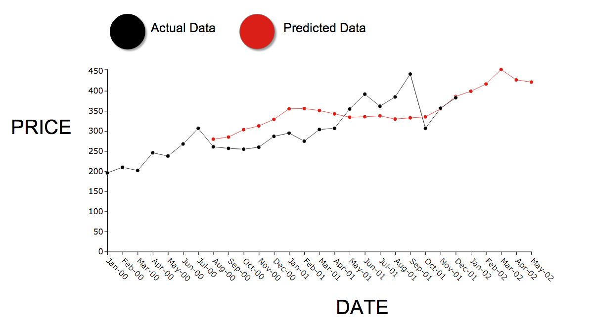
Example

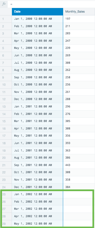
In the following example we have price values per month over a two year period. Let's try to predict the first 5 months of the third year using [double exponential smoothing.]

Add five additional rows in the date column to better visualize the results for 5 months of future predictions.
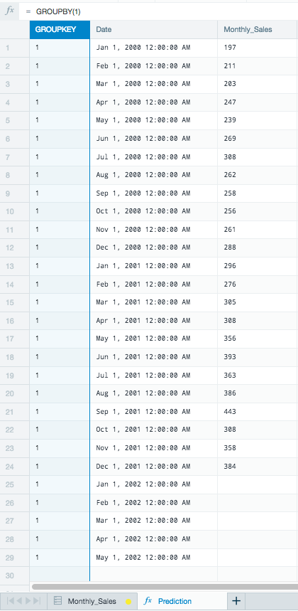
Create a new worksheet in your Workbook by duplicating the source sheet.
Create a group key using GROUPBY(1).
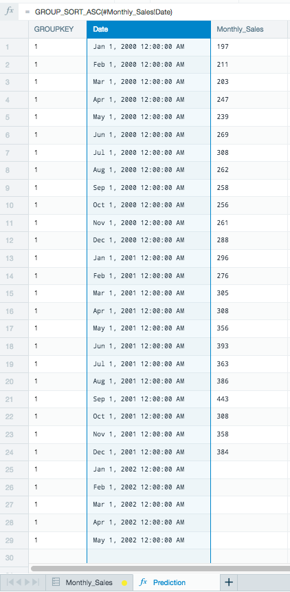
Sort the timeline using GROUP_SORT_ASC(#Monthly_Sales!Date).
Click the Fx button on the formula line to display the Formula Builder and select GROUP_HOLT_WINTERS.
Use the monthly sales column for the value's argument.

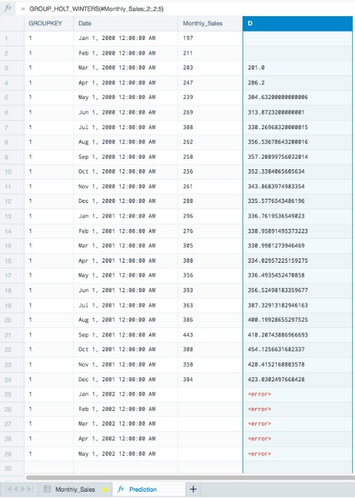
As this example uses a small data set, the alpha and beta arguments are set low at 0.2.

With a larger data set, you can set the alpha and beta arguments higher as there is more data to allocate into making the predictions. Allocating too many data resources with a smaller data set can make predictions less reliable as there is not enough steady data to understand trends.

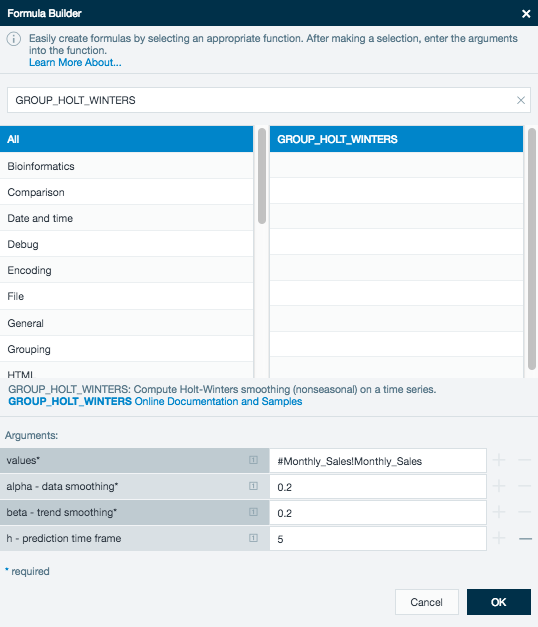
The Formula bar looks like this for your predicted values:

GROUP_HOLT_WINTERS(#Monthly_Sales;0.2;0.2;5)

There are two missing values for the rows, GROUP_HOLT_WINTERS needs these two values to compute the first prediction. Also, these predictions are 5 points in the future and currently don't match up with the date row.

To correct this, modify your Formula bar to:

GROUP_PREVIOUS(IF(ISNULL(#Monthly_Sales);null;GROUP_HOLT_WINTERS(#Monthly_Sales;0.2;0.2;5));5)

This uses the functions GROUP_PREVIOUS to move the predictions 5 rows down to line up with the correct date. This also uses the function ISNULL to correct the error for the missing values in the rows with no values.

The sheet now displays the predicted data using the Holt-Winters exponential smoothing method.

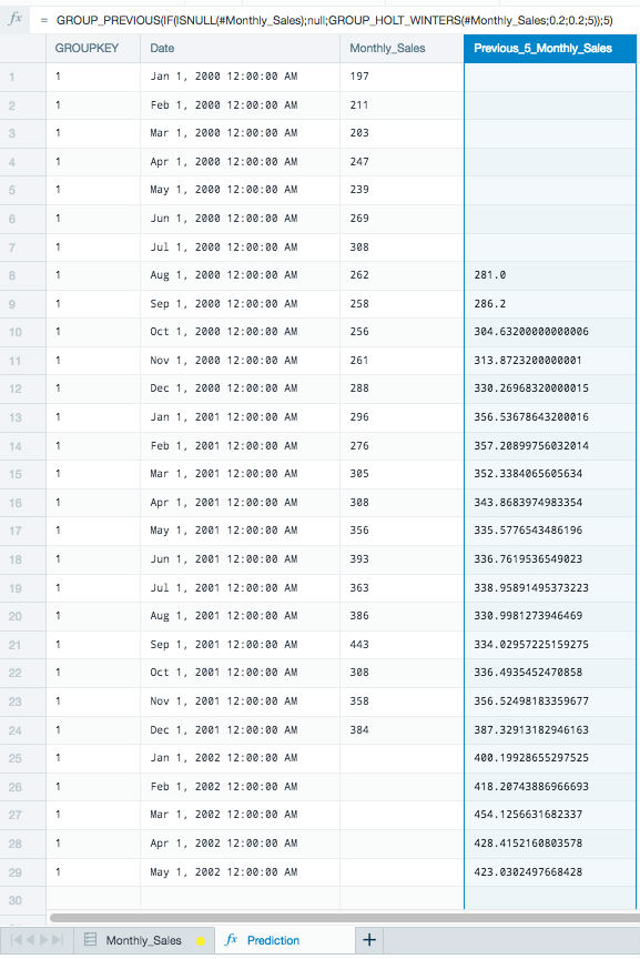
Your finished Workbook displays the full date range, the original values, and the predicted values.

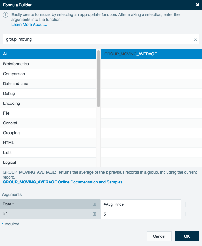
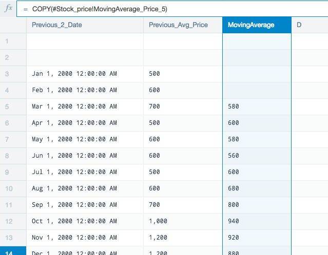
GROUP_MOVING_AVERAGE#

Syntax#

GROUP_MOVING_AVERAGE(<number>;[<number>])

Values: time series values

K: number of past values to compute the moving average from

Description#

This function smooths a time series by applying a simple moving average of the past k values. Smoothing a time series helps remove random noise and leave the user with a general trend. You might use [[GROUP_HOLT_WINTERS](#group_holt_winters) for exponential smoothing.

Example

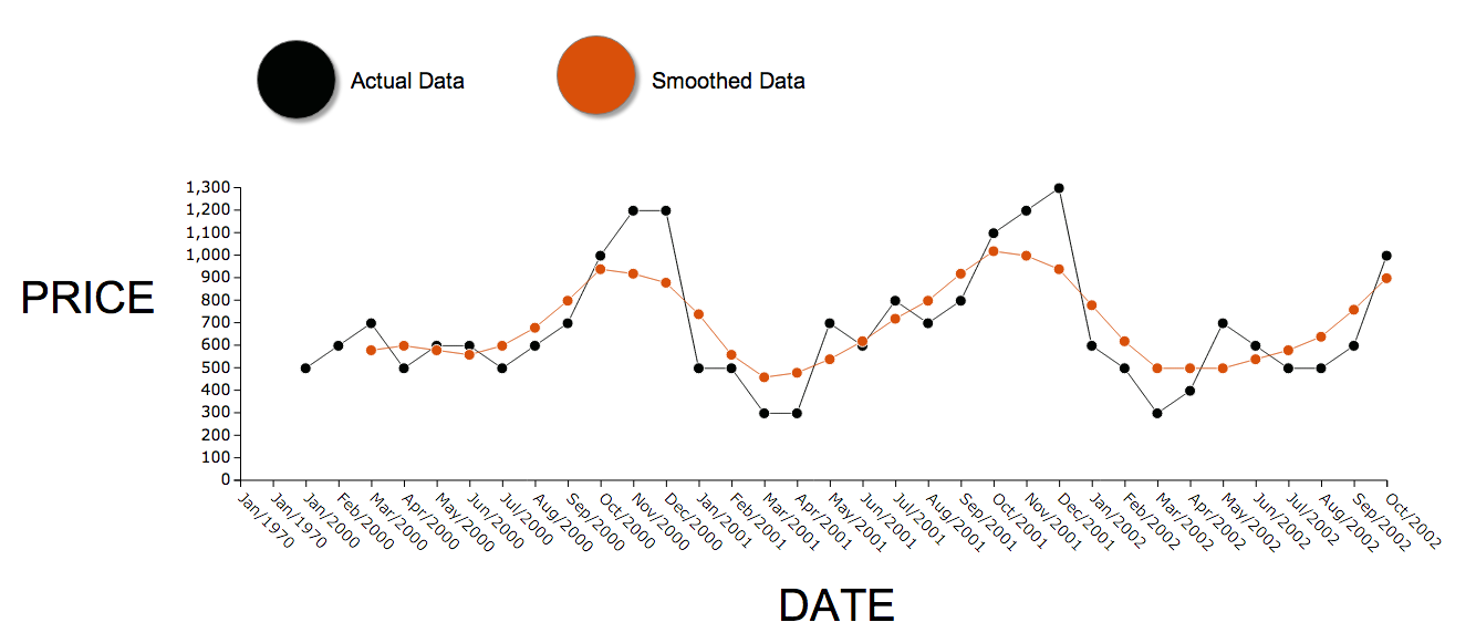
In the following example you have average stock price values per month over a three year period. Try to smooth the data to find the general trend.

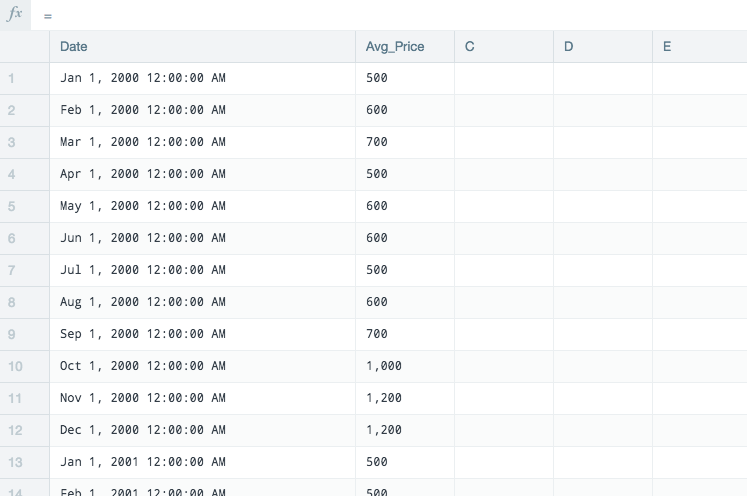
Next, duplicate this source into a calculation sheet in order to work on it.

Click an empty column to bring up the Formula Builder and select GROUP_MOVING_AVERAGE.

Use the Avg_Price as the Data and set the k at 5. This uses each previous 5 months to create a smoothed average for each data record.

The first record in the column MovingAverage_Price_5 is an average of the first 5 records of Avg_Price.

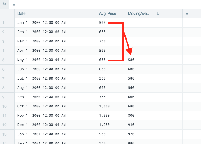
As the Moving_Average_Price_5 records are the average of the previous 5 Avg_Price records, the Moving_Average needs to match to the median of the Date and Ave_Price.

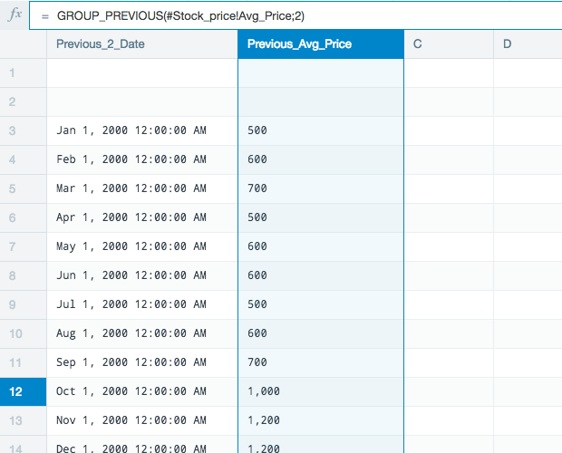
Create a new sheet and click the first open column to bring up the Formula Builder. Select GROUP_PREVIOUS to shift the Date column down two rows.

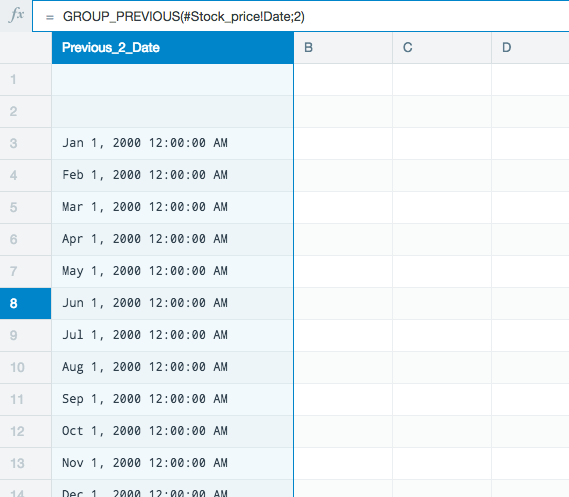
Use the same GROUP_PREVIOUS function to shift the Avg_Price down by two rows.

Finally, COPY the MovingAverage_Price_5 into the sheet.

The moving average values are now properly aligned with the median date and price the moving average is based on.

Real World Examples of Group Series Functions#

Here we show a few examples of the power of using group series functions and how they can be used in your analyses:

Click stream analysis with session ID#

Group series functions can be used for click stream analysis:

Group according to the session key.
Sort all values within each session by the timestamp.
Generate click paths using the URLs.

For example, suppose you have the following input data:

Input1

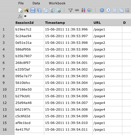
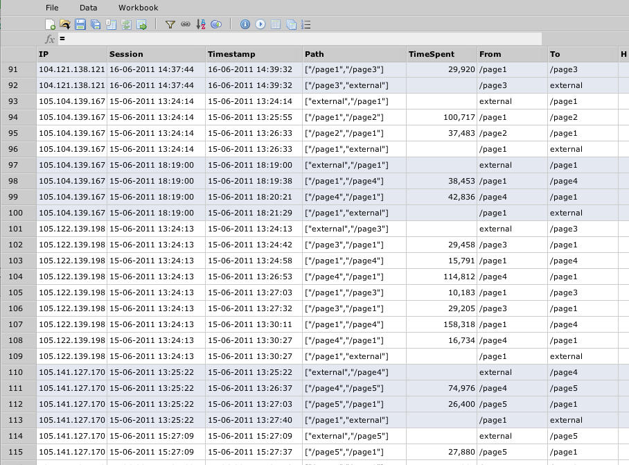
Generating click stream information is done within one formula sheet:

=GROUPBY(#Input!SessionId)
=GROUP_SORT_ASC(#Input!Timestamp)
=GROUP_PATH_CHANGES(#Input!URL)
=GROUP_DIFF(#Timestamp)
=JSON_ELEMENT(#Path;0)
=JSON_ELEMENT(#Path;1)

The result of this sheet looks like this:

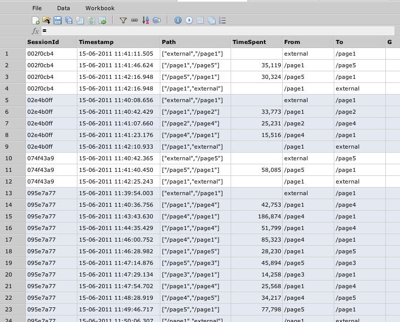
After that, you can do whatever analysis is required, for example, you could do the following:

Find the page where users spend most time on by:
1. Doing GROUPBY(#ClickStream!From) and GROUPMEDIAN(#ClickStream!TimeSpent).
2. Sorting by TimeSpent.
Find the page where a user most often leaves the application by:
1. Filtering all records, where #ClickStream!To == "external".
2. Doing GROUPBY(#From) and GROUPCOUNT().
3. Sorting by count in descending order.
Find most often page transitions by:
1. Doing GROUPBY(#ClickStream!From), GROUPBY(#ClickStream!To) and GROUPCOUNT().
2. Sorting by count in descending order.

Click stream analysis without session ID#

In many cases you might not have a session ID in your data so you can't group on a session as easily. But usually it's possible to extract a session from your data. For example, if you have IP addresses and timestamps in your server log, you could assume that for each IP address a new session begins when there is a gap of more than x minutes between one and the next log entry. This means that the request is coming from the same machine, but it's probably a different session. The GROUPBYGAP function helps you determine the session information.

For example, suppose you have the following input data:

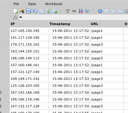
Generating click streams can be done within one formula sheet:

=GROUPBY(#Input!IP)
=GROUPBYGAP(#Input!Timestamp;10m)
=#Input!Timestamp
=GROUP_PATH_CHANGES(#Input!URL)
=GROUP_DIFF(#Timestamp)
=JSON_ELEMENT(#Path;0)
=JSON_ELEMENT(#Path;1)

The result of this sheet looks like this:

Market basket analysis#

Another use case for group series analysis is determining which products have been bought together in one transaction in order to do recommendations. To do this analysis, you can use a GROUP_PAIR function that creates all pairs of a value within one group.

Suppose you have a data structure such as this:

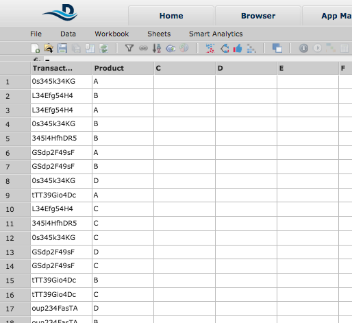
You can now do the following analysis:

=GROUPBY(#Input!Transaction)
    -The GROUPBY function groups all the transactions of the same value together.
=GROUP_PAIR(#Input!Product)
    -The GROUP_PAIR function can be used after a GROUPBY function to return all pairs of values of each GROUPBY value in a list.
=LISTELEMENT(#Product_Pairs;0)
=LISTELEMENT(#Product_Pairs;1)
    -The LISTELEMENT functions are used to extract the first and second elements of the list into separate columns.

The result sheet looks like this:

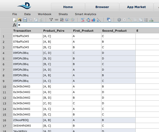
Next, you can aggregate on pairs to see which pairs occur most often in one transaction.

Grouping Functions#

Group Series Functions#

GROUPACCUMULATE#

Syntax#

Description#

GROUPBOTTOMN#

Syntax#

Description#

GROUPBY#

Syntax#

Description#

GROUPBYBIN#

Syntax#

Description#

GROUPBYCUSTOMBIN#

Syntax#

Description#

GROUPBYGAP#

Syntax#

Description#

GROUPCOMBIN#

Syntax#

Description#

GROUPPREDICTIVEWINDOWS#

Syntax#

Description#

GROUPROWNUMBER#

Syntax#

Description#

GROUPSESSIONS#

Syntax#

Description#

GROUPTOPN#

Syntax** **#

Description#

GROUPUNIQUES#

Syntax#

Description#

GROUP_DIFF#

Syntax#

Description#

GROUP_PAIR#

Syntax#

Description#

GROUP_PATH#

Syntax#

Description#

GROUP_PATH_CHANGES#

Syntax#

Description#

GROUP_PREVIOUS#

Syntax#

Description#

GROUP_SORT_ASC#

Syntax#

Description#

GROUP_SORT_DESC#

Syntax#

Description#

Aggregate Functions#

GROUPAND#

Syntax#

Description#

GROUPANOVA#

Syntax#

Description#

GROUPANY#

Syntax#

Description#

GROUPAVERAGE#

Syntax#

Description#

GROUPCONCAT#

Syntax#

Description#

GROUPCONCATDISTINCT#

Syntax#

Description#

GROUPCOUNT#

Syntax#

Syntax #